Properties of the Complexity Coefficients

Introduction

Darkhovsky and Piryatinska have conjectured that for a constant generating process the complexity coefficients time series generated by that process are constant. More concretely, we tested if, for a constant Hölder class of functions, the complexity coefficients are also constant.

A Hölder-\(\alpha\) class of functions is a set of functions with a bounded rate of change indexed by the parameter \(\alpha\). Specifically, a Hölder continuous function \(f(x)\) is one that satisfies \[ | f(x + h) - f(x)| < C|h|^{\alpha}, \] for positive constants \(C\), \(\alpha\).

Three of the simulations used in our previous tests have parameters that determine the Hölder-\(\alpha\) class of the time series generated by the process or function – fractional Brownian Motion (fBm), the random Weierstrass function, and the Cauchy process. For each of these random processes, and for the Weierstrass function, the Hölder class and fractal dimension are determined by the same parameter. The complexity coefficients were estimated on time series generated over a range of parameters for each function or process. In addition to computing the complexity coefficients, fractal dimension was estimated using a variogram-based estimator¹.

For all process except for the random Weierstrass function, the mean of the complexity coefficient \(B\) changed linearly with the Hölder class of the time series and with the time series’ estimated fractal dimension. Here we present the results from the Weierstrass function and the Cauchy process.

Weierstrass Function

The Weierstrass function is well-known example of a continuous but nowhere differentiable function. The function can be written: \[ W_{\alpha}(x) = \sum_{n=0}^{\infty}b^{-n\alpha}\cos(b^n \pi x). \] In this form, the single parameter \(\alpha\) is the Hölder class for the function and \(2-\alpha\) is the functions fractal dimension². Graphs of the Weierstrass function where \(b = 2\) and for several \(\alpha\) parameters are shown below.

# Weierstrass function without random phase
library(dplyr)

if(!exists("from_cache")){
  from_cache = TRUE
}

prefix = "holder_notrandom"
len = 1000

set.seed(seed)
alpha <- seq(0.1, 0.99, length.out = 20)
reps = 1
if(from_cache) {
  xs     <- readRDS(cache_file("weierstrass_xs", prefix)) 
  emeans <- readRDS(cache_file("weierstrass_ecomp", prefix))
  emc    <- readRDS(cache_file("weierstrass_emc", prefix))
  fdmc    <- readRDS(cache_file("weierstrass_fdmc", prefix))
  fdmeans    <- readRDS(cache_file("weierstrass_fdmean", prefix))

} else {
  # generate set of weierstrass functions for each alpha
  ws <- lapply(alpha, function(x) tssims::weierstrass(a = x, random = FALSE))
  xs <- replicate(reps, sapply(ws, function(w) tssims::gen(w)(1000)))
  xs <- xs[3:997, , ]
  # takes 3 dimensional array, with the third dimension the parameter
  ecomp <-  apply(xs, 2, ecomp_cspline)
  fd <- apply(xs, 2, fd_variogram)
  emeans <- lapply(ecomp, function(x) data.frame(A = x$A, B = x$B)) %>% 
            do.call(rbind, .)
  fdmeans <- lapply(fd, function(x) data.frame(fd = x$fd)) %>% 
            do.call(rbind, .)

  emeans$alpha <- alpha
  names(emeans) <- c("A", "B", "alpha")
  save_cache(xs, "weierstrass_xs", prefix)
  save_cache(emeans, "weierstrass_ecomp", prefix)
  save_cache(emc, "weierstrass_emc", prefix)
  save_cache(fdmeans, "weierstrass_fdmean", prefix)
  save_cache(fdmc, "weierstrass_fdmc", prefix)
}

# Plot time series and boxplots of coeffcients
cols <- seq(1, 19, by = 2)
cols = c(3, 8, 16)
# alpha[cols]

# Plot a single example from fbm with different parameters
plot.ts(xs[,cols], main = "Weierstrass function", col = viridis::viridis(30)[3])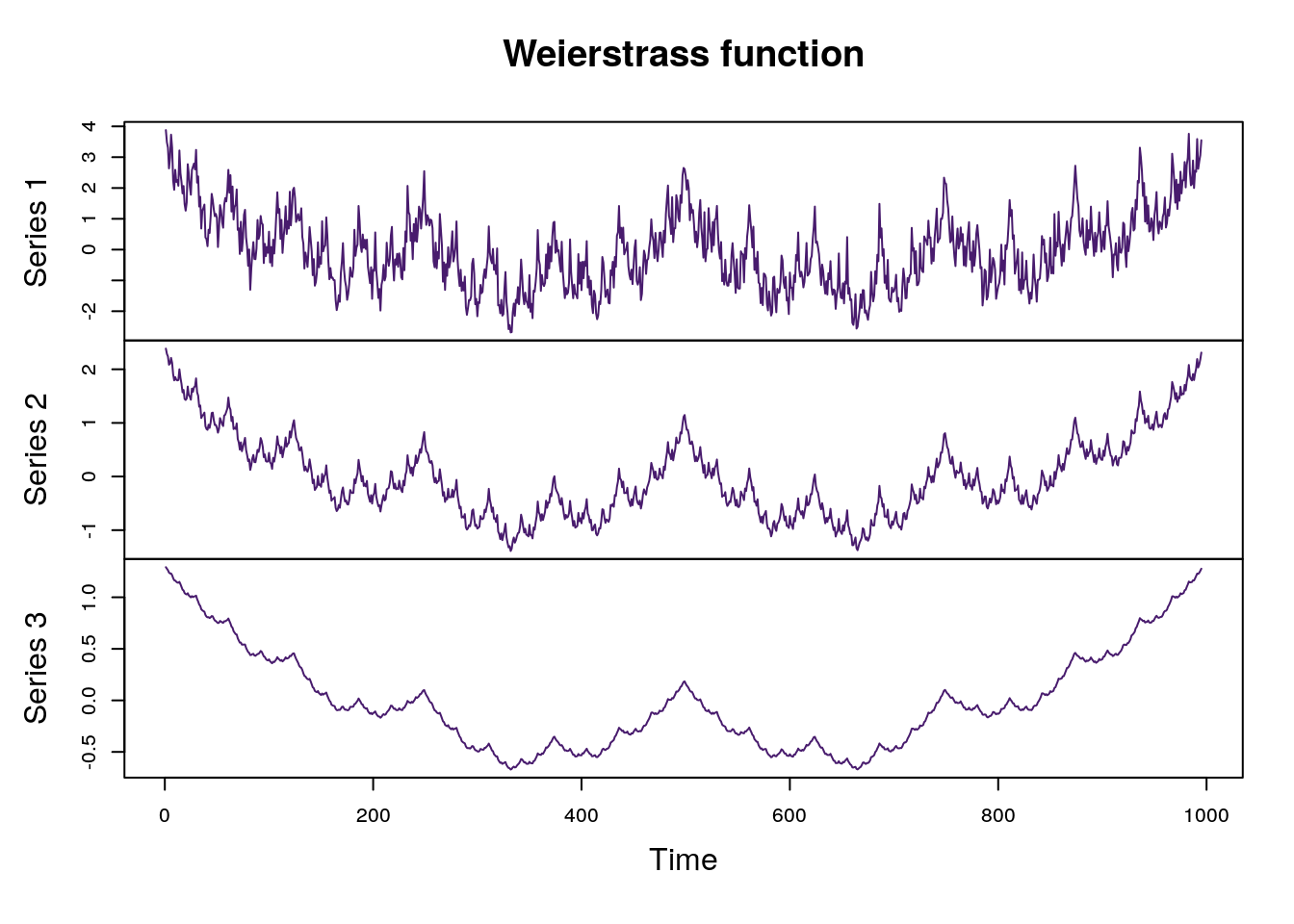

Plot of Weierstrass function with alpha parameters (0.2, 0.42, 0.8)

The complexity coefficients and fractal dimension were estimated for 20 values of \(\alpha\). The results plotted below show that the all both complexity coefficients and fractal dimension change linearly with the \(\alpha\) parameter.

  par(mfrow = c(1, 3))
  plot(alpha[1:19],  emeans[1:19, 1], 
     xlab = "Alpha", 
       ylab = "A", 
       cex = 1.2,
       col = eegpalette(1)[1]
       )
  
  plot(alpha[1:19], emeans[1:19, 2], 
       xlab = "Alpha", 
       ylab = "B", 
       cex = 1.3,
       col = eegpalette(1)[2]
       )
  plot(alpha[1:19], fdmeans[1:19, 1], 
       xlab = "Alpha", 
       ylab = "Fractal Dimension", 
       cex = 1.3, 
       col = eegpalette(1)[3]
       )

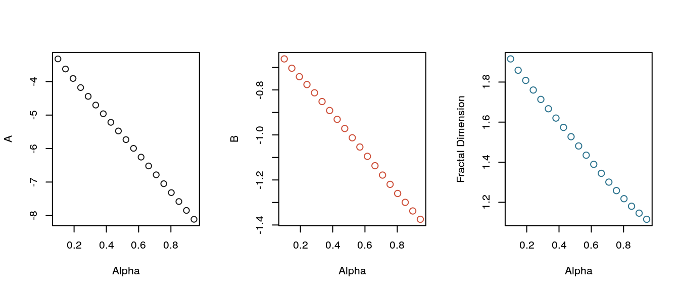
Complexity coefficients and fractal dimension plotted against the Weierstrass parameter alpha.

  knitr::read_chunk("../code/holder-cauchy-plots.R")

Cauchy process

The Hurst parameter is a measure of the long range dependence of a random process. Fractional Brownian motion has a single parameter that determines both the Hölder class andfractal dimension of its sample paths and the Hurst parameter. The Cauchy process, on the other hand, has two parameters which separately determine the fractal dimension and Hurst parameter of sample paths of the process.

The Cauchy process is defined in terms of its correlation function \[ c(h) = (1 + |h|^{\alpha})^{-\beta/\alpha}, \hspace{1em} h \in \mathbb{R}. \]

For \(\alpha \in (0, 2]\) the fractal dimension of the Cauchy process is \[ D = 2 - \frac{\alpha}{2}. \]

And for \(\beta \in (0,1)\) its Hurst parameter is \[ H = 1 - \frac{\beta}{2}. \]

The plot below shows the Cauchy process on a 3 \(\times\) 3 grid of parameters. Fractal dimension (and the Hölder class) are constant on the columns. The plots are labeled with their theoretical Hurst parameter and the estimated complexity coefficient \(B\).

  library(ecomplex)
  library(dplyr)
  library(ggplot2)
  library(ggthemes)
  
  if(!exists("from_cache")){
    from_cache = TRUE
  }
  
  prefix = "cauchy"
  len = 150
  reps = 50
  set.seed(2017)
  
  alpha <- seq(0.1, 1.3, length.out = 3) 
  beta <- seq(0.01, .7, length.out = 3)
  
  alpha_to_fd <- function(alpha) alpha + 1 - alpha/2
  beta_to_hurst <- function(beta) 1 - beta/2
  
  ab <- expand.grid(alpha, beta)
  fh <- cbind(alpha_to_fd(ab[,1]), beta_to_hurst(ab[,2]))
  names(ab) <- c("alpha", "beta")
  names(fh) <- c("Fractal_dim", "Hurst")
  
  
  ws <- apply(ab, 1, function(x) tssims::cauchy(alpha = x[1], beta = x[2]))
  xs <- lapply(ws, function(w) tssims::gen(w)(len)) %>% 
        do.call(cbind, .) %>% 
        data.frame
  
  comps <- lapply(xs, function(x) tsfeats::get_features(x, tsfeats::ecomp_cspline)) %>% 
           do.call(rbind, .) %>% round(., 2)
  
  
  names(xs) <- paste0("Complexity 'B'=", comps[,2], " , ", "Hurst=", round(fh[,2], 2))
  plot_ts(xs, ncol = 3, col = viridis::viridis(30)[3])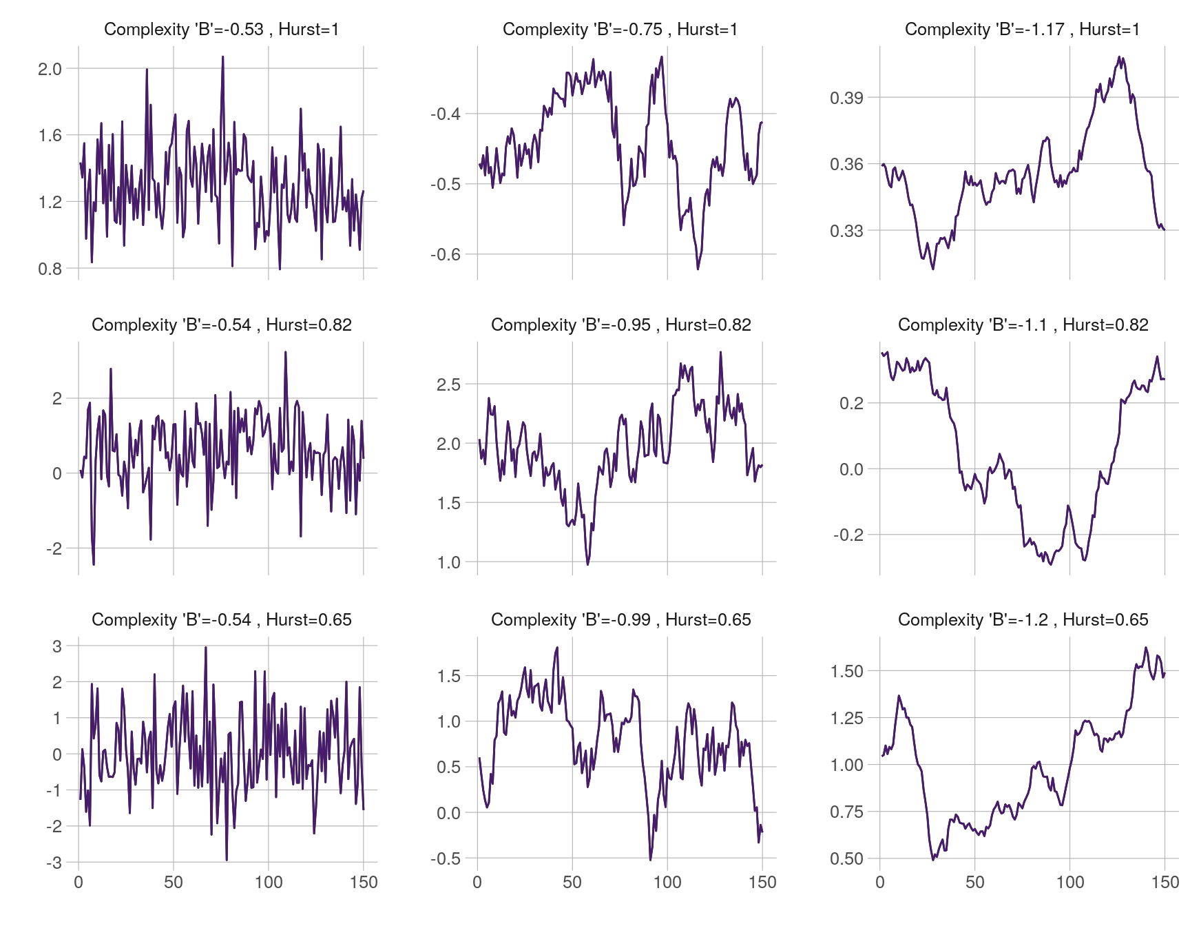

Plot of Cauchy process for a grid of parameters.

30 samples were generated for each parameter combination on a 10 \(\times\) 10 grid. The plots below show the estimates for the complexity coefficients and fractal dimension plotted separately against the \(\alpha\) parameter and \(\beta\) parameter. The plots show the complexity coefficient \(B\) and the fractal dimension estimator change linearly with \(\alpha\) but are largely unaffected by the changes in the Hurst parameter.

  knitr::read_chunk("../code/holder-cauchy.R")

  library(ecomplex)
  library(dplyr)
  library(ecomplex)
  library(tsfeats)
  
  set.seed(2017)
  
  if(!exists("from_cache")){
    from_cache = TRUE
  }
  len <- 500
  reps <- 30
  prefix <- "cauchy"
  
  alpha <- seq(0.01, 1.99, length.out = 10) 
  beta <- seq(0.01, 1.5, length.out = 10)
  ab <- expand.grid(alpha, beta)
  
  if(!from_cache){
    ws <- apply(ab, 1, function(x) tssims::cauchy(alpha = x[1], beta = x[2]))
    xs <- replicate(reps, sapply(ws, function(w) tssims::gen(w)(len)))
  
    emc <- mc_features(xs, tsfeats::ecomp_cspline)
    fdmc <- mc_features(xs, tsfeats::fd_variogram)
    hmc <- mc_features(xs, tsfeats::hurst_pracma)
  
    save_cache(emc, "ecoeff", prefix) 
    save_cache(fdmc, "fd", prefix) 
    save_cache(hmc, "hurst", prefix) 
    save_cache(xs, "xs", prefix)
  } else{
    xs  <- readRDS(cache_file("xs", prefix)) 
    emc<- readRDS(cache_file("ecoeff", prefix))
    fdmc <- readRDS(cache_file("fd", prefix))
    hmc <- readRDS(cache_file("hurst", prefix))
  }
  
  emean <- mc_stat(emc, mean)
  varmean  <- mc_stat(emc, var)
  fdmean <- mc_stat(fdmc, mean) 
  hmean <- mc_stat(hmc, mean)
   
  cols = c(22, 25, 29)
  
  # Plot a single example from fbm with different parameters
  
  # pdf(file.path(getwd(), paste0("figures/", prefix, "-plot.pdf")), 
      # width = 5, height = 4)
  # plot.ts(xs[, cols, 1], main = "Cauchy process")
  # dev.off() 
  
  coeffA <- lapply(emc, function(x) x[,1]) %>% 
            do.call(cbind, .) %>%
            data.frame
  
  coeffB <- lapply(emc, function(x) x[,2]) %>% 
            do.call(cbind, .) %>%
            data.frame
  
  coeffFD <- lapply(fdmc, function(x) x[,1]) %>%          
             do.call(cbind, .) %>%
             data.frame
  
  colnames(coeffA) <- paste0(rep(round(alpha, 2), 10))
  colnames(coeffB) <- paste0(rep(round(alpha, 2), 10))
  colnames(coeffFD) <- paste0(rep(round(alpha, 2),10))
  
  
  ab_df  <- cbind(emean, ab, fdmean, hmean, varmean)
  names(ab_df) <- c("A", "B", "Alpha", "Beta", "fd", "hurst")
  
  # pdf(file.path(getwd(), paste0("figures/", prefix, "alpha-scatterplots.pdf")), 
      # width = 9, height = 4)
  par(mfrow = c(1, 3))
  with(ab_df, plot(Alpha, A,  col = eegpalette(1)[1], cex = 1.2))
  with(ab_df, plot(Alpha, B,  col = eegpalette(1)[2], cex = 1.2))
  with(ab_df, plot(Alpha, fd, ylab = "Fractal Dimension", col = eegpalette(1)[3], cex = 1.2))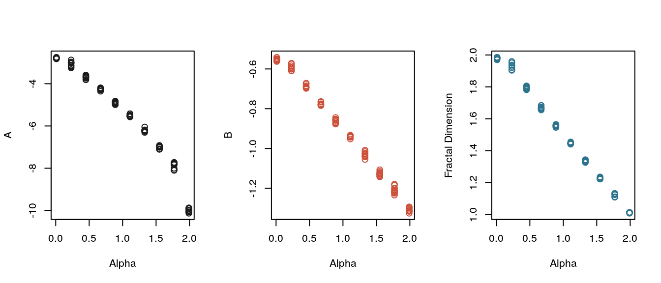

Plot of complexity coefficients and fractal dimension of the Cauchy processes generated from a grid of parameters.

  # dev.off()
  
  
  # pdf(file.path(getwd(), paste0("figures/", prefix, "beta-scatterplots.pdf")), 
  #     width = 9, height = 4)
  par(mfrow = c(1, 3))
  with(ab_df, plot(Beta, A,  col = eegpalette(1)[1]) )
  with(ab_df, plot(Beta, B,  col = eegpalette(1)[2]) )
  with(ab_df, plot(Beta, fd, ylab = "Fractal Dimension", col = eegpalette(1)[3]) )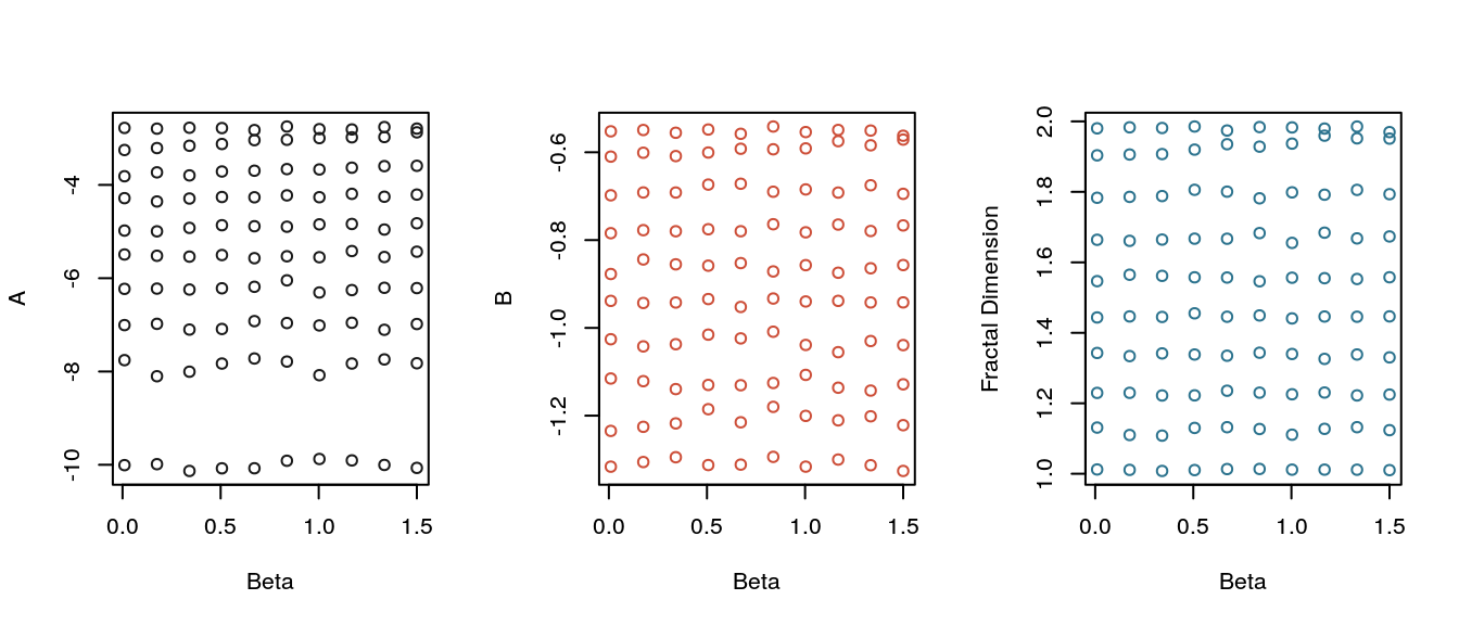

Plot of complexity coefficients and fractal dimension of the Cauchy processes generated from a grid of parameters.

  # dev.off() 

Discussion

Similar results held for fBm but not for the random Weierstrass function. For each process tested in this section, the complexity coefficient \(B\) behaved like the variogram-based fractal dimension estimator. It’s likely that the complexity coefficient \(B\) is an estimator of fractal dimension. One approach to proving this is would be to restrict the proof, for example, to stationary Gaussian processes and to simple polynomial or even linear approximation.

Session information

sessionInfo()

R version 3.4.1 (2017-06-30)
Platform: x86_64-pc-linux-gnu (64-bit)
Running under: Ubuntu 14.04.5 LTS

Matrix products: default
BLAS: /usr/lib/libblas/libblas.so.3.0
LAPACK: /usr/lib/lapack/liblapack.so.3.0

locale:
 [1] LC_CTYPE=en_US.UTF-8       LC_NUMERIC=C              
 [3] LC_TIME=en_US.UTF-8        LC_COLLATE=en_US.UTF-8    
 [5] LC_MONETARY=en_US.UTF-8    LC_MESSAGES=en_US.UTF-8   
 [7] LC_PAPER=en_US.UTF-8       LC_NAME=C                 
 [9] LC_ADDRESS=C               LC_TELEPHONE=C            
[11] LC_MEASUREMENT=en_US.UTF-8 LC_IDENTIFICATION=C       

attached base packages:
[1] stats     graphics  grDevices utils     datasets  methods   base     

other attached packages:
[1] tsfeats_0.0.0.9000 ggthemes_3.4.0     ggplot2_2.2.1     
[4] ecomplex_0.0.1     dplyr_0.7.2        eegcomplex_0.0.0.1

loaded via a namespace (and not attached):
 [1] reshape2_1.4.2           lattice_0.20-35         
 [3] splines_3.4.1            colorspace_1.2-6        
 [5] fArma_3010.79            htmltools_0.3.6         
 [7] yaml_2.1.14              rlang_0.1.1             
 [9] pracma_2.0.7             ForeCA_0.2.4            
[11] glue_1.1.1               withr_1.0.2             
[13] sp_1.2-5                 splus2R_1.2-1           
[15] bindrcpp_0.2             plyr_1.8.4              
[17] bindr_0.1                stringr_1.2.0           
[19] timeDate_3012.100        munsell_0.4.3           
[21] fBasics_3011.87          commonmark_1.2          
[23] gtable_0.2.0             timeSeries_3022.101.2   
[25] devtools_1.13.2          gmwm_2.0.0              
[27] memoise_1.1.0            evaluate_0.10.1         
[29] labeling_0.3             knitr_1.16              
[31] highr_0.6                Rcpp_0.12.12            
[33] scales_0.4.1             backports_1.0.5         
[35] abind_1.4-3              sapa_2.0-2              
[37] gridExtra_2.2.1          fracdiff_1.4-2          
[39] digest_0.6.12            stringi_1.1.5           
[41] grid_3.4.1               rprojroot_1.2           
[43] fractaldim_0.8-4         quadprog_1.5-5          
[45] tools_3.4.1              magrittr_1.5            
[47] ifultools_2.0-4          lazyeval_0.2.0          
[49] pdc_1.0.3                tibble_1.3.3            
[51] randomForest_4.6-12      pkgconfig_2.0.1         
[53] MASS_7.3-45              xml2_1.1.1              
[55] RandomFieldsUtils_0.3.25 RandomFields_3.1.50     
[57] tssims_0.0.0.9000        assertthat_0.2.0        
[59] rmarkdown_1.6            roxygen2_6.0.1          
[61] viridis_0.3.4            R6_2.2.2                
[63] git2r_0.19.0             compiler_3.4.1