Project overview
Last updated: 2017-07-26
- Simulation and Approximation Methods
- Properties of the Complexity Coefficients
- Seizure Prediction
- Computing the Complexity Coefficients
The \(\varepsilon\)-complexity of a continuous function is, roughly speaking, the amount of information needed to reconstruct that function within an absolute error \(\varepsilon\). The theory and procedure for estimating \(\varepsilon\)-complexity was introduced by Darkhovsky and Piryatinska1. In previous work, the complexity coefficients have been shown to be useful features for the segmentation and classification of time series2.
The purpose of these analyses was three-fold:
To improve the estimation of the complexity coefficients by enlarging the set of approximation methods used in the estimation procedure.
To explore the relation between the complexity coefficients, the Hölder condition and fractal dimension.
An application of the complexity coefficients to the segmentation and classification of EEG.
Along with an overview of the results of each of these analyses we outline the procedure for estimating the complexity coefficients.
library(devtools)
load_all()
knitr::read_chunk("../code/eeg-segment-plot.R")
par(mar = c(0, 0, 2, 0))
library(ggplot2)
library(dplyr)
library(viridis)
library(ecomplex)
prefix = "eeg"
seed = 2017
# Derived features. 30 Trials : 6 channels : 15 features
feature_df <-readRDS(cache_file("mod_all_features", prefix))
# Load meta data
trial_df <- readRDS(cache_file("mod_trial_segments", "eeg"))
df <- do.call(rbind, feature_df) %>%
cbind(., trial_df) %>%
dplyr::filter(., window == 240)
df$trial <- 1:26
ch = 1; colnums = c(5:9, 13:15); tnum = 8
dfch <- df[[ch]][[tnum]]
res <- palarm(dfch$ecomp.cspline_B)
seg_plot <- function(startn, stopn, title ="", ...){
segcol = adjustcolor("tomato3", 0.9)
pal = c("gray20", segcol, viridis::viridis(256)[c(1, 30, 60, 90, 120)])
plot(dfch$ecomp.cspline_B + 3,
type = 'l',
col = adjustcolor("gray20", 0.6),
lwd = 2,
lty = 1,
cex = 0.5,
ylim = c(0,2.2),
xlim = c(0,120),
xlab = "Time",
yaxt = "n",
ylab = "",
main = title,
...)
lines(res$means + 3, type = 'l', xlim=c(0,120), col=segcol, lwd=2, lty= 1 )
for(k in startn:stopn) lines(dfch[ , 4 + k] + 0.5*(k-startn),
lwd = 2,
col = pal[k + 2])
for(k in res$kout) abline(v = k, col = segcol, lwd = 1.5, lty = 2)
}
# pdf(file.path(getwd(), paste0("figures/", prefix, "-segment-plot.pdf")),
# width = 9, height = 4)
par(mfrow = c(1,1), mar = c(1,1,1,1))
seg_plot(3,5, xaxt = "n")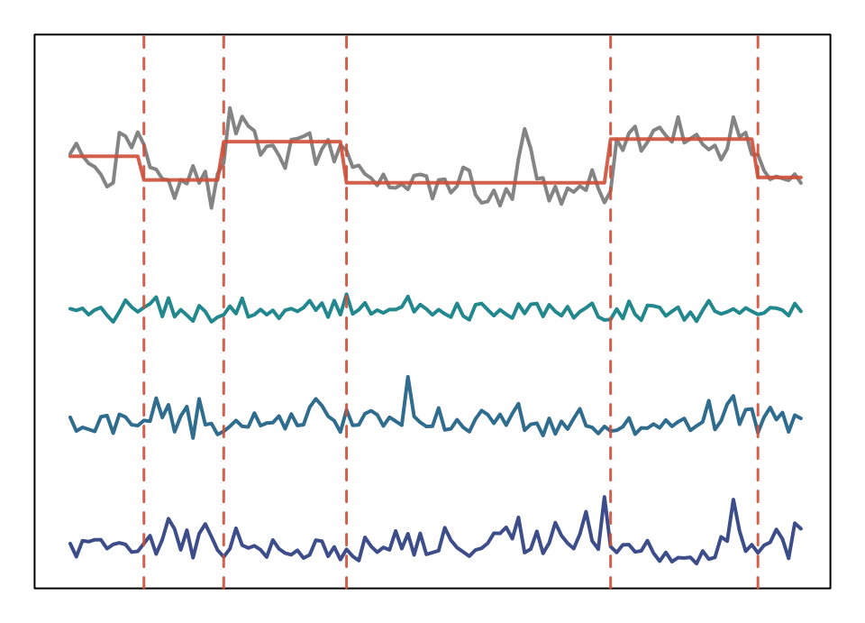
Segmentation of spectral freatures based complexity coefficient change points
Credits
These poject pages were developed with the help of the workflowr package.