Simulation Examples
Nathanael Aff
2017-05-10
Last updated: 2017-07-26
Code version: 26dff77
Introduction
The \(\varepsilon-\)complexity of a time series is computed by successively downsampling and approximating the original time series. The initial implementation of the \(\varepsilon-\)complexity procedure used piecewise polynomials as the approximation method. We implemented the procedure in the R language using three approximation methods, B-splines, cubic splines, and interpolating subdivision. The spline methods use existing libraries. The interpolating subdivision was implemented based on Sweldens1.
The purpose of adding additional approximation methods was to improve the performance of the complexity coefficients in segmentation and classification tasks. We found that the most accurate approximation method – B-splines with a large number of basis elements – did not perform better than cubic splines or the lifting method in classification tasks. Because all methods performed similarly, the computationally efficient implementation of cubic splines was used in later applications.
knitr::read_chunk("../code/sim-example.R")library(ggplot2)
library(dplyr)
library(ggthemes)
library(tssims)
library(ecomplex)
library(tsfeats)
library(fArma)
# Generate simulations
devtools::load_all()
prefix = "sim"
seed = 1
set.seed(seed)
len <- 200
gs <- tssims::sim_suite()
gs <- lapply(gs, function(x) lapply(x, tssims::jitter_params))
ys1 <- lapply(gs$group1, function(mod) tssims::gen(mod)(len))
ys2 <- lapply(gs$group2, function(mod) tssims::gen(mod)(len))
df <- data.frame(do.call(cbind, c(ys1, ys2)) %>% apply(., 2, normalize))
names(df) <- tssims::sim_names()
names(df) <- c("ARMA 1", "Logistic 1", "Weierstrass 1", "Cauchy 1", "FARIMA 1", "FBM 1",
"ARMA 2", "Logistic 2", "Weierstrass 2", "Cauchy 2", "FARIMA 2", "FBM 2")
palette(eegpalette()[c(1,3,4)])
nsims <- length(names(df))
id <- factor(rep(rep(c(1,2), each = 200), 6))
dfm <- df %>% tidyr::gather(variable, value)
dfm$variable <- factor(dfm$variable)
plot_fit <- function(res, fname){
xlab = "log( S )"; ylab = "log( epsilons )"
plot(
log(res$S),
log(res$epsilons),
yaxt = "n",
pch = 2,
ylab = ylab,
xlab = xlab,
main = fname
)
abline(res$fit, lwd = 1.6, col = eegpalette()[3])
}
gp <- ggplot(dfm, aes(x = rep((1:len), nsims), y = value)) +
labs(x = "", y = " ")
gp + geom_line(size = 0.6, alpha = 0.85, colour = id) +
facet_wrap(~variable, scales = "free_y", ncol = 2) +
# scale_color_manual(values = eegpalette()[c(1,3)]) +
theme_minimal2() 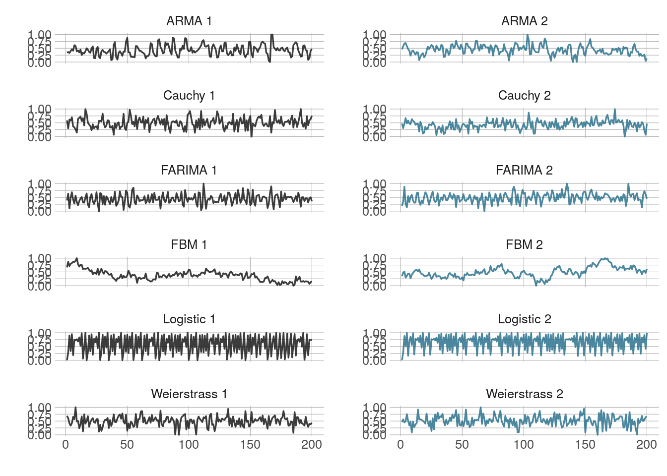
Single time series from each simulation group.
save_plot("jitter_timeseries", prefix)Diagnostic plots
In the theory developed by Piryatinska and Darkhovsky2, the \(log-log\) regression of approximation errors taken at each downsampling level \(S\) should be roughly linear. (An outline of the estimation procedure is here.) The two parameters defining this linear fit are the complexity coefficients.The implementation of the three approximation methods was checked to determine that this linear relationship held for a set our set of simulations. The plot shows the diagnostic plots for the interpolating subdivision method.
# Plot example fit for each function


par(mfrow = c(2,3))
fits <- apply(df[1:6], 2, ecomplex::ecomplex, method = "lift")
names(fits) <- c("ARMA", "Logistic", "Weierstrass", "Cauchy", "FARIMA", "FBM")
out <- Map(plot_fit, fits, names(fits))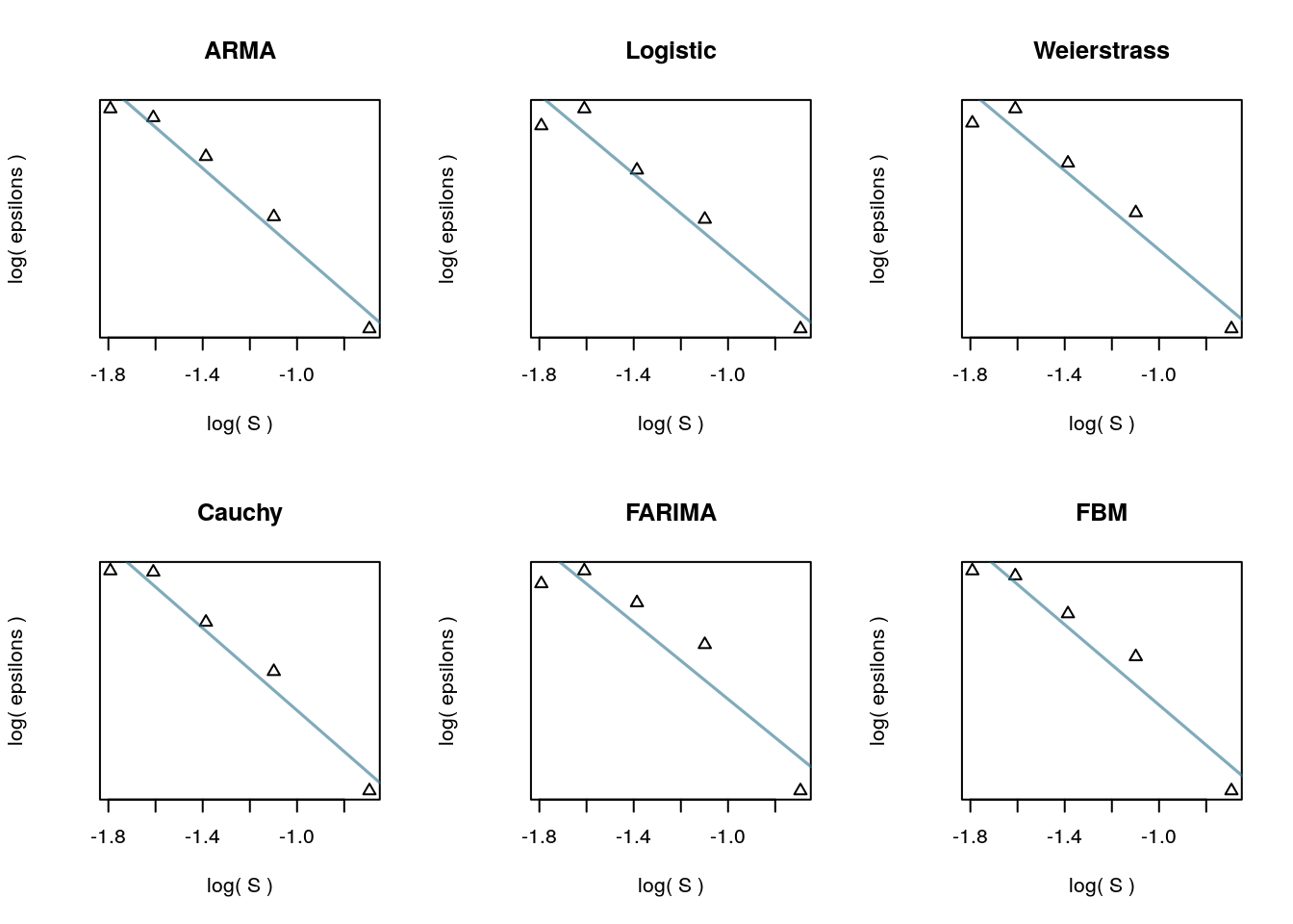
Diagnostic plots for interpolating subdivision.
Approximation method performance
A plot of the simulations in the feature space of the two complexity coefficients shows that the complexity coefficients generated by each method lie in roughly the same area in the coefficient space. The same processes – ARMA, logistic map, and fBM – also appear linearly separable for each method. The plot shows that, roughly, all three methods produce similar estimations of the complexity coefficients.
knitr::read_chunk("../code/ecomplex-plot-feature-space.R")devtools::load_all()
library(ggplot2)
library(dplyr)
prefix = "ecomplex"
sim_df1 <- readRDS(cache_file("approx_types1", prefix))
# sim_df <- readRDS(cache_file("approx_types", prefix))
sim_df1 <- sim_df1 %>% dplyr::filter(variable != "ecomp_all_B")
sim_df1$id2 <- as.factor(rep(c(1,2,1,3,1,4,1,5,1,6,1,7), each = 30))
# pal <- c("gray10", viridis::viridis(60)[c(5,10,15,20,25,30)])
pal <- eegpalette(0.7)[c(1,3)]
gp <- ggplot(data = sim_df1, aes(x = value, y = yvalue))
gp + facet_grid(~ variable, scales = "free_y") +
geom_point(aes(colour = id, shape = fnames), size = 2) +
scale_color_manual(values = pal) +
theme_minimal() +
labs(x = "A", y = "B")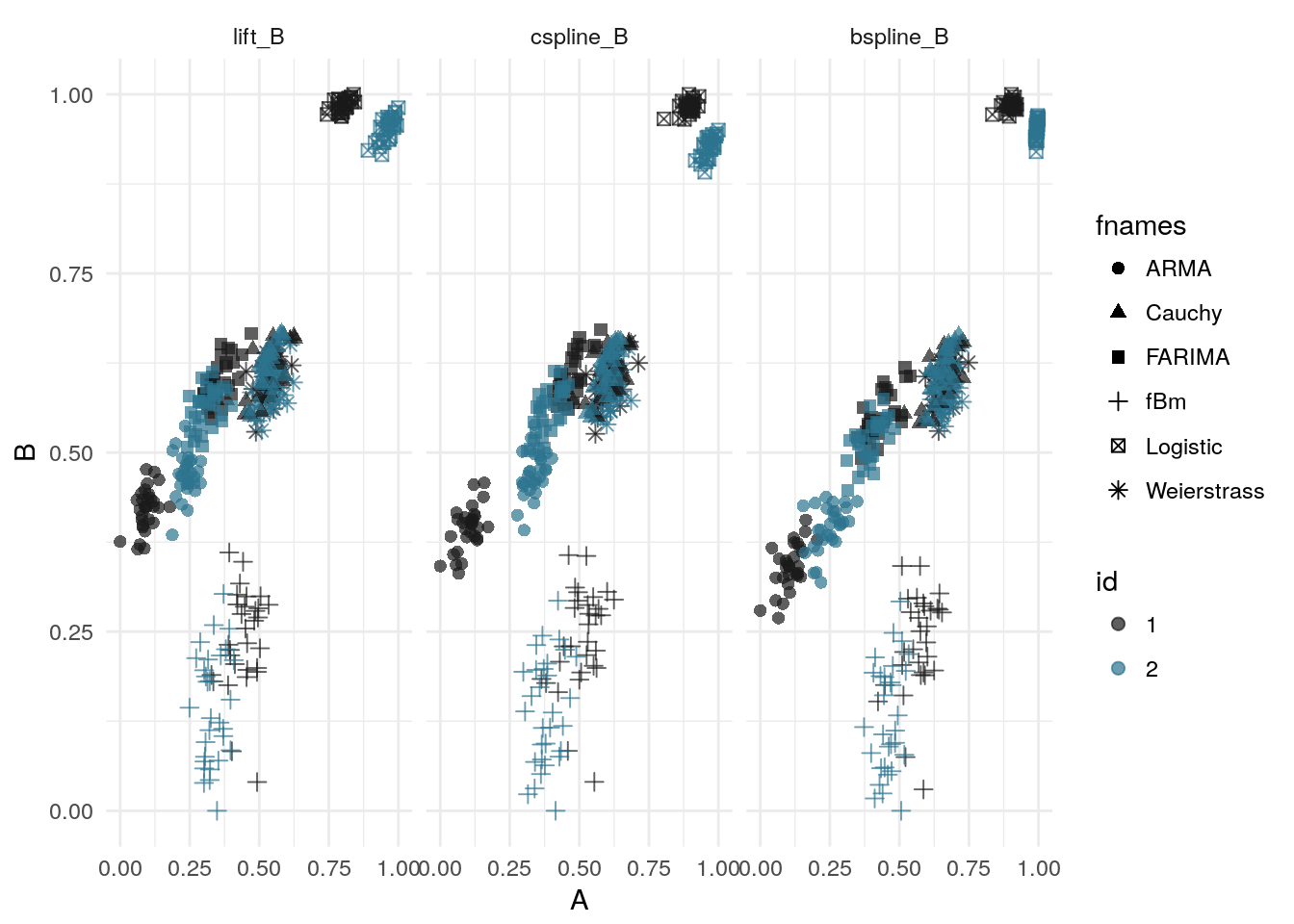
# save_plot("approx-feature-space", prefix)For the following test two groups were formed consisting of 30 simulations of each random process or function. Each process had an initial set of parameters and samples of the process were generated by randomly perturbing these parameters within a small window. As the table above shows, the B-spline method produced the lowest total approximation error. The ‘Combined’ method, which used the smallest approximation at each downsample level, mirrors the B-spline results.
  devtools::load_all()
  prefix = "ecomplex"

  err_means <- readRDS(cache_file("all_errs", prefix))
  rf_errs <- readRDS(cache_file("rf_errs", prefix))

  err_means <- data.frame(err_means)
  names(err_means) <- names(rf_errs)
  row.names(err_means) <- row.names(rf_errs)
knitr::kable(err_means, caption = 'Approximation error for each method.')| Lift | Cspline | Bpsline | Combined | |
|---|---|---|---|---|
| ARMA | 0.100 | 0.104 | 0.066 | 0.066 |
| Logistic | 0.308 | 0.326 | 0.198 | 0.198 |
| Weierstrass | 0.108 | 0.116 | 0.070 | 0.070 |
| Cauchy | 0.118 | 0.124 | 0.076 | 0.076 |
| FARIMA | 0.134 | 0.142 | 0.086 | 0.086 |
| fBm | 0.036 | 0.042 | 0.024 | 0.024 |
The complexity coefficients were used as features in a random forest classifier, the same classifier we used in later applications. No approximation method was clearly dominant but the methods with higher approximation errors performed as well or better than the B-spline method. All three approximation methods are similar – essentially, the basis elements reproduce lower order polynomials – so the result is not too suprising. On the other hand, the results do indicate that improved approximation does not necessarily lead to improved performance in classification tasks that use the complexity coefficients as classifiers.
Additional work could test whether these results hold for simulations run over a larger range of parameters, or if different classifiers yield similar results.
knitr::kable(rf_errs, caption = 'Classification error for each approximation method.')| Lift | Cspline | Bpsline | Combined | |
|---|---|---|---|---|
| ARMA | 0.033 | 0.000 | 0.067 | 0.067 |
| Logistic | 0.000 | 0.000 | 0.017 | 0.000 |
| Weierstrass | 0.524 | 0.427 | 0.411 | 0.427 |
| Cauchy | 0.492 | 0.556 | 0.476 | 0.476 |
| FARIMA | 0.330 | 0.297 | 0.313 | 0.330 |
| fBm | 0.199 | 0.215 | 0.215 | 0.182 |
Session information
sessionInfo()R version 3.4.1 (2017-06-30)
Platform: x86_64-pc-linux-gnu (64-bit)
Running under: Ubuntu 14.04.5 LTS
Matrix products: default
BLAS: /usr/lib/libblas/libblas.so.3.0
LAPACK: /usr/lib/lapack/liblapack.so.3.0
locale:
[1] LC_CTYPE=en_US.UTF-8 LC_NUMERIC=C
[3] LC_TIME=en_US.UTF-8 LC_COLLATE=en_US.UTF-8
[5] LC_MONETARY=en_US.UTF-8 LC_MESSAGES=en_US.UTF-8
[7] LC_PAPER=en_US.UTF-8 LC_NAME=C
[9] LC_ADDRESS=C LC_TELEPHONE=C
[11] LC_MEASUREMENT=en_US.UTF-8 LC_IDENTIFICATION=C
attached base packages:
[1] stats graphics grDevices utils datasets methods base
other attached packages:
[1] eegcomplex_0.0.0.1 bindrcpp_0.2 fArma_3010.79
[4] fBasics_3011.87 timeSeries_3022.101.2 timeDate_3012.100
[7] tsfeats_0.0.0.9000 ecomplex_0.0.1 tssims_0.0.0.9000
[10] ggthemes_3.4.0 dplyr_0.7.2 ggplot2_2.2.1
loaded via a namespace (and not attached):
[1] Rcpp_0.12.12 sapa_2.0-2
[3] lattice_0.20-35 tidyr_0.6.3
[5] splus2R_1.2-1 assertthat_0.2.0
[7] rprojroot_1.2 digest_0.6.12
[9] R6_2.2.2 plyr_1.8.4
[11] RandomFields_3.1.50 backports_1.0.5
[13] evaluate_0.10.1 ForeCA_0.2.4
[15] pracma_2.0.7 highr_0.6
[17] rlang_0.1.1 lazyeval_0.2.0
[19] gmwm_2.0.0 fracdiff_1.4-2
[21] rmarkdown_1.6 labeling_0.3
[23] devtools_1.13.2 splines_3.4.1
[25] stringr_1.2.0 munsell_0.4.3
[27] compiler_3.4.1 pkgconfig_2.0.1
[29] htmltools_0.3.6 tibble_1.3.3
[31] gridExtra_2.2.1 roxygen2_6.0.1
[33] quadprog_1.5-5 randomForest_4.6-12
[35] withr_1.0.2 MASS_7.3-45
[37] commonmark_1.2 grid_3.4.1
[39] gtable_0.2.0 git2r_0.19.0
[41] magrittr_1.5 pdc_1.0.3
[43] scales_0.4.1 fractaldim_0.8-4
[45] stringi_1.1.5 reshape2_1.4.2
[47] viridis_0.3.4 sp_1.2-5
[49] xml2_1.1.1 tools_3.4.1
[51] glue_1.1.1 abind_1.4-3
[53] yaml_2.1.14 colorspace_1.2-6
[55] memoise_1.1.0 knitr_1.16
[57] bindr_0.1 RandomFieldsUtils_0.3.25
[59] ifultools_2.0-4