Seizure Prediction
Nathanael Aff
2017-07-10
Last updated: 2017-07-26
Code version: 26dff77
Introduction
The EEG signal exhibit abrupt changes in their statistical distribution and functional behavior. The procedure for estimating complexity coefficients was developed, in part, as a model free way of detecting changes in the underlying generating mechanism. We assume that such regime changes are reflected in changes in the complexity coefficients. With that in mind, we used change points in the complexity coefficients to segment the EEG signal. The goal was to compute features on more homogeneous segments rather than on arbitrary partitions.
EEG from several optogenetically modified epileptic mice were used to predict a seizure response to a laser stimulus. A single set of features including relative bandpower and several nonlinear features were used to predict the response. Several models were built using features calcuated on both uniform segmentation of the raw EEG and on segmetation based on change points in the complexity coefficients. Models using the complexity based partitions performed no better than the uniform partition schemes.
The EEG came from 4 intercranial EEG channels and 2 local field potential(LFP) sensors. The LFP data capture the electrical potential of a small group of neurons located in the thalamus. All models were based on single channel EEG channels. We compare the features predictive of a seizure outcome for each channel and the feature distribution associated with seizure and non-seizure responses. Gamma and beta levels in the LFP channels were the strongest predictor of a seizure responses.
There are several inherent flaws in the data that are discussed in more detail below. All seizures come from a single mouse and seizure responses were recorded in most cases following a previous seizure.
Classification models
The plot below illustrates a partition of spectral features based on change points in the complexity coefficient \(B\). In total, 6 segmentation models were used: segmentation based on complexity coefficients \(A\) and \(B\) – individually and combined – and three models using uniform partitions.
 devtools::load_all()
  knitr::read_chunk("../code/eeg-segment-plot.R")
library(ggplot2)
library(dplyr)
library(viridis)
library(ecomplex)
prefix = "eeg"
seed = 2017
# Derived features. 30 Trials : 6 channels : 15 features
feature_df <-readRDS(cache_file("mod_all_features", prefix))
# Load meta data
trial_df <- readRDS(cache_file("mod_trial_segments", "eeg"))
df <- do.call(rbind, feature_df) %>%
cbind(., trial_df) %>%
dplyr::filter(., window == 240)
df$trial <- 1:26
ch = 1; colnums = c(5:9, 13:15); tnum = 8
dfch <- df[[ch]][[tnum]]
res <- palarm(dfch$ecomp.cspline_B)
seg_plot <- function(startn, stopn, title ="", ...){
segcol = adjustcolor("tomato3", 0.9)
pal = c("gray20", segcol, viridis::viridis(256)[c(1, 30, 60, 90, 120)])
plot(dfch$ecomp.cspline_B + 3,
type = 'l',
col = adjustcolor("gray20", 0.6),
lwd = 2,
lty = 1,
cex = 0.5,
ylim = c(0,2.2),
xlim = c(0,120),
xlab = "Time",
yaxt = "n",
ylab = "",
main = title,
...)
lines(res$means + 3, type = 'l', xlim=c(0,120), col=segcol, lwd=2, lty= 1 )
for(k in startn:stopn) lines(dfch[ , 4 + k] + 0.5*(k-startn),
lwd = 2,
col = pal[k + 2])
for(k in res$kout) abline(v = k, col = segcol, lwd = 1.5, lty = 2)
}
# pdf(file.path(getwd(), paste0("figures/", prefix, "-segment-plot.pdf")),
# width = 9, height = 4)
par(mfrow = c(1,2), mar = c(2,2,2,2), cex.main = .9)
seg_plot(1,2, "Segmentation of Delta, Theta")
seg_plot(3,5, "Segmentation of Alpha, Beta, Gamma")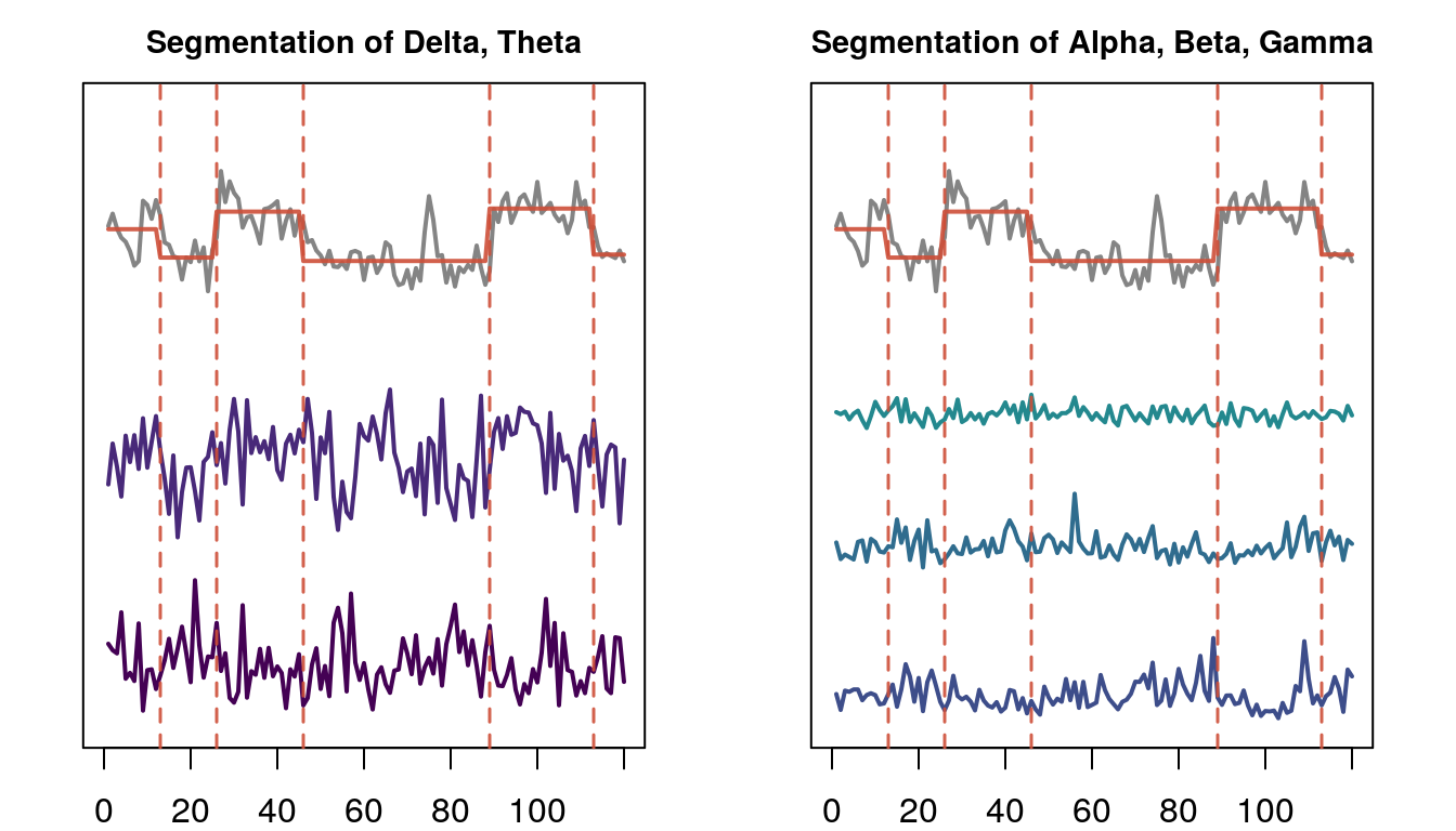
Segmentation of trial one based on the complexity coefficient \(B\). Only spectral features are shown.
There were 26 trials with 9 seizure responses. The underlying classifier is a random forest. The classification performance reported in the table below is the mean balanced accuracy based on 30 iterations of 5-fold cross-validation.
The mean balanced accuracy for each model and channel is reported below. All models performed better on channels 1 and 2: these are local field potential(LFP) channels which record the activity of a small set of neurons in the thalamus. The regular partition models of 8 and 15 partitions performed better across most channels.
knitr::read_chunk("../code/eeg-tables.R") library(dplyr)
prefix = "eeg"
vecmeans <- readRDS(cache_file("vecmeans", prefix))
ABmeans <- readRDS(cache_file("ABmeans", prefix))
ABacc <- ABmeans %>% lapply(., function(x) x["Balanced.Accuracy", ]) %>%
bind_rows(.) %>%
data.frame
vecacc <- vecmeans %>% lapply(., function(x) x["Balanced.Accuracy", ]) %>%
bind_rows(.) %>%
data.frame
combacc <- rbind(ABacc, vecacc)
names(combacc) <- paste0("ch", 1:6)
methods <- c("A", "B", "A+B", "8", "15", "30")
row.names(combacc) <- methods
combacc <- apply(combacc, 2, round, digits = 2)
names(combacc) <- paste0("Channel ", 1:6)
knitr::kable(combacc, caption = "Balanced accuracy of each models and channel combination.")| ch1 | ch2 | ch3 | ch4 | ch5 | ch6 | |
|---|---|---|---|---|---|---|
| A | 0.81 | 0.78 | 0.70 | 0.74 | 0.56 | 0.63 |
| B | 0.84 | 0.76 | 0.71 | 0.73 | 0.61 | 0.63 |
| A+B | 0.79 | 0.74 | 0.73 | 0.72 | 0.55 | 0.59 |
| 8 | 0.86 | 0.83 | 0.74 | 0.73 | 0.73 | 0.77 |
| 15 | 0.84 | 0.84 | 0.75 | 0.71 | 0.72 | 0.75 |
| 30 | 0.79 | 0.77 | 0.75 | 0.77 | 0.74 | 0.73 |
Data
The EEG data was collected from mice with a genetic mutation that makes them prone to epilepsy. The mice are also genetically modified to allow for direct stimulation of neurons by a laser pulse.
Data was gathered from 13 distinct time periods during which a laser stimulus was applied between one to four times. There were 26 trials in total. The 4-minute segments preceding the stimulus was used to predict outcomes.
  devtools::load_all()
  knitr::read_chunk("../code/eeg-plot.R")
eeg <- readRDS(cache_file("eegsnip", prefix = "eeg"))
# dim(eeg)
fs <- 1220.703
plot_range <- function(a,b){
oldpar = par()
par(mfrow = c(6, 1), mar = c(1, 1, 1, 1))
for(k in 1:6){
plot(eeg[k, a:b],
type = 'l',
col = "gray30",
lwd = 1.5,
axes = FALSE,
frame.plot = FALSE)
}
}
secs = 8
a = 37000
b = a + fs*secs
plot_range(a,b)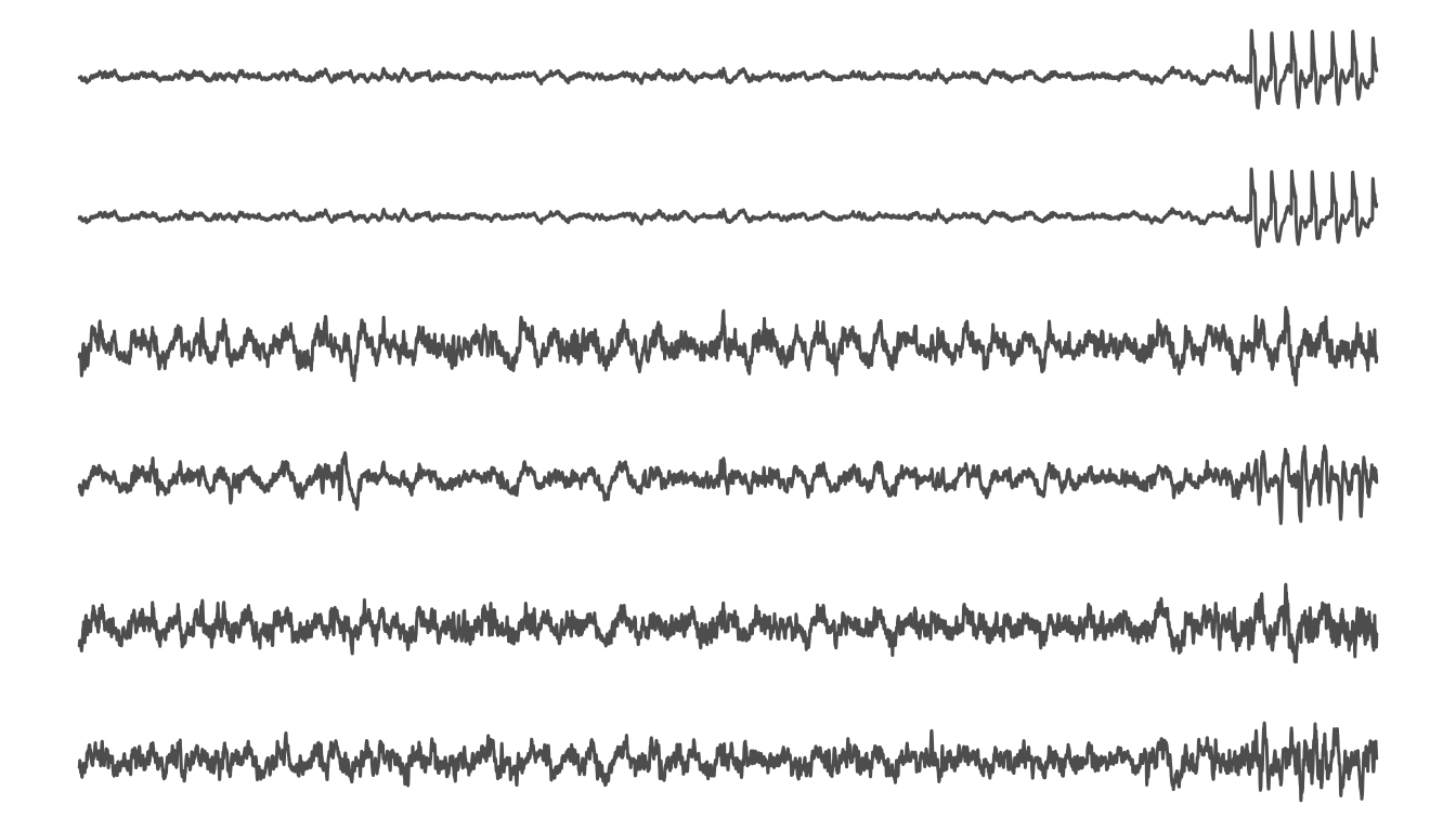
8 second window of EEG inclduing the start appplication of a laser stimulus.
While we were able to prediction seizures on with a relatively high degree of accuracy – over 80% for some channels, there are significant limitations to the data. First and foremost, all seizures came from an individual mouse. We can only make limited inferences about features related to seizure responses without additional data. Variations in the features could be specific to the biology or measurement devices particular to that mouse.
Seizures also occured mainly in the same series of trials. A plot below shows a shematic diagram of the trials. Each bar represents a single trial. Filled boxes indicate a trial period and green bars indicate an application of the stimulus. Most seizures occured in a trial following a previous seizure: these are indicated by blue boxes.
Again, features associated with seizures may simply be features that occur following a seizure, not preceeding it.
knitr::read_chunk("../code/eeg-trial-plot.R") library(dplyr)
from_cache = TRUE
plot_trial <- function(df_){
plot(
y,
xlim = c(0, max_end),
ylim = c(-0.5, 0.5),
lwd = 0.2,
lty = 3,
col = "gray40",
type = 'l',
xlab = '',
ylab = '',
yaxt = 'n',
xaxt = 'n'
)
for(k in (1:dim(df_)[1])){
rcol <- keycols[df_$col_key[k]]
if(df_$col_key[k]!=4){
count <<- count + 1
rect((
df_$stim_start[k]-240),
-0.5,
df_$stim_start[k],
0.5,
col = rcol,
border = "transparent")
text(df_$stim_start[k]-120, 0, paste0(count),
cex = 1.3,
col = "gray90"
)
}
abline(v = (df_$stim_start[k]+1), col = "chartreuse3", lwd = 3)
}
}
count = 0
metadf <- readRDS(cache_file("windows2", "meta"))
# Fix errror:
metadf$col_key[13] <- 4
trial_keys <- unique(metadf$key)
max_end <- max(metadf$stim_end)
x <- (0:max_end)
y <- rep(0, length(x))
keycols <- eegpalette()
# pdf(file.path(getwd(), paste0("figures/", prefix, "-param-plots-notrandom.pdf")),
# width = 9, height = 4)
par(mfrow = c(8,2), mar = c(1, 0.5, 1, 0.5), cex.axis = 1.4, cex.lab = 1.4)
for(k in 1:length(trial_keys)){
df_ <- metadf %>% dplyr::filter(key == trial_keys[k])
plot_trial(df_)
}
plot(1, type = 'n', axes = "FALSE")
legend(x = "center", inset = 0,
c("No response", "1st response ", "2nd response"),
col = keycols, pch = 15, cex = 1.3, horiz = TRUE)
plot(1, type = 'n', axes = "FALSE")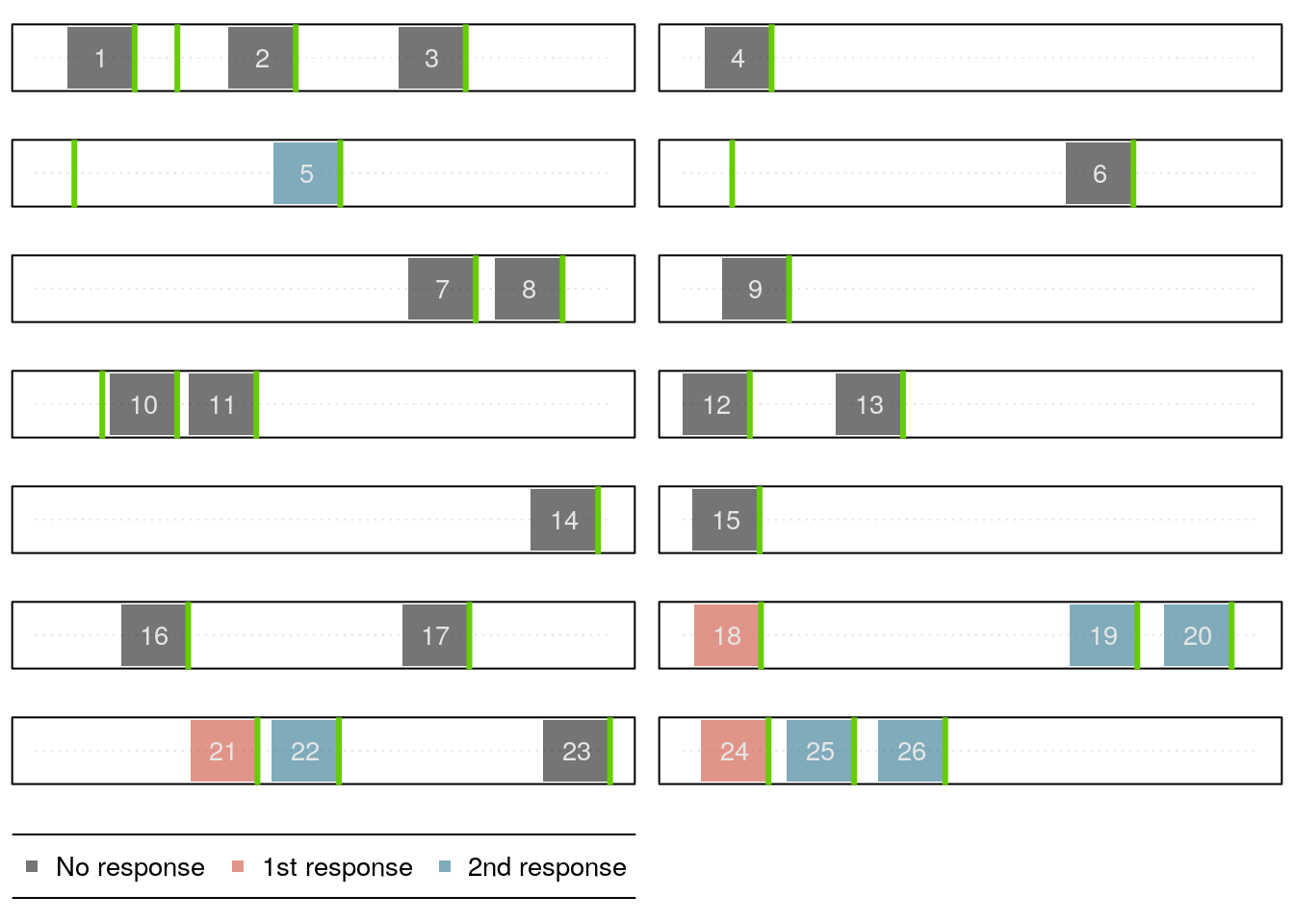
Schematic of the trial time periods. A seizures is indicated as a ‘repsonse’ and initial seizures and secondary seizures are indicated by color.
# dev.off()The plot below shows the probability of seizure as estimated by a single model for each trial. Pink and blue indicate seizure responses. For most trials the model separates seizure and non-seizure trials fairly well. However, the initial seizure responses are much closer to the threshold than the later seizure trials.
knitr::read_chunk("../code/eeg-cv-ch1-plot.R") library(ggplot2)
prefix = "eeg"
palette(eegpalette())
meta_df <- readRDS(cache_file("windows2", "meta"))
predict <- readRDS(cache_file("cv_results_ch_1", "eeg") )
predict_df <- predict$df
colkey <- predict_df$trial_type <- meta_df %>%
dplyr::filter(window == 240) %>%
dplyr::select(col_key)
colkey <- colkey[[1]]
# colkey[colkey == 3] <- 2
thresholds <- readRDS(cache_file("cvthresholds", prefix))
tnames <- paste0("Trial ", 1:26)
tnames <- factor(tnames, levels = tnames)
names(predict_df) <- c("response","probability", "trialnum", "ground")
# Edited : Seizure vs No seizure
ggplot(predict_df, aes( x = tnames, y = probability)) +
geom_point(stat='identity', aes(col=as.factor(colkey)), size= 4) +
scale_color_manual(name="",
labels = c("No response", "Seizure response", "2nd response"),
values = eegpalette()) +
labs(y = "Probability", x = "") +
coord_flip() +
geom_hline(yintercept=thresholds[[1]], colour = "chartreuse3") +
theme_bw() +
theme(text = element_text(size= 16),
axis.text.x = element_text(size = 16),
panel.background = element_rect(fill = "transparent", colour = NA),
# panel.background = element_blank(),
plot.background = element_blank(),
legend.background = element_rect(fill = "transparent", colour = NA))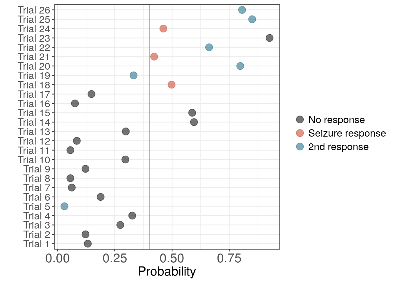
Probability of seizure for model built on channel 1 using complexity coefficients.
palette("default")Feature importance
Despite variations in classification performance, variable importance was similar across models. The variable importance for two models plotted in the figure below. Both models were build on data from channel 1. On the left is the model segmented on the combined complexity coefficients A and B. On the right is a model with 8 uniform partitions.
knitr::read_chunk("../code/eeg-classify-roc-import.R") library(ggplot2)
library(dplyr)
library(ecomplex)
library(randomForest)
library(tssegment)
library(caret)
library(corrplot)
prefix = "eeg"
seed = 2017
chs = 1:6
from_cache = TRUE
window = 240
len = window/2
feature_df <-readRDS(cache_file("mod_all_features", "eeg"))
trial_df <- readRDS(cache_file("mod_trial_segments", "eeg"))
# Select trials with 4 minute windows and
# combine feature data frames with metadata
df <- do.call(rbind, feature_df)
df <- df %>% cbind(trial_df)
df <- dplyr::filter(df, window == 240)
df$trial <- 1:26
# Run cross validation segmenting on a single feature and
# channel.
run_on_feat <- function(df_, ch, feat, m = 5, byname = TRUE){
colnums = c(5:9, 13:18)
if(byname){
means_df <- segment_on_cols(df_, ch, cols = feat, m = m)
} else {
means_df <- segment_on_cols(df_, ch, vec = feat, new_vec = TRUE, m = m)
}
cat("Number of segments: ", dim(means_df)[1], "\n")
cat("Using channel: ", ch, "\n")
cm <- run_cv(means_df, df$response, ch, colnums, TRUE)
}
# Compute importance
varnames <- c("Delta", "Theta", "Alpha", "Beta", "Gamma",
"Variance", "Hurst", "Spectral Entropy")
if(!from_cache){
feat <- c("ecomp.cspline_B")
resAB_raw <- resvec_raw <- list()
for(ch in 1:6){
resAB_raw[[ch]] <- run_on_feat(df, ch, feat, m = 3, byname = TRUE)
resvec_raw[[ch]] <- run_on_feat(df, ch, (1:120), m = 10, byname = FALSE)
}
save_cache(resAB_raw, "resAB_raw", "eeg")
save_cache(resvec_raw, "resvec_raw", "eeg")
} else {
resAB_raw <- readRDS(cache_file("resAB_raw", "eeg"))
resvec_raw <- readRDS(cache_file("resvec_raw", "eeg"))
}
ABimport <- lapply(resAB_raw, function(x) x$importance) %>%
do.call(rbind, .) %>%
data.frame
vecimport <- lapply(resvec_raw, function(x) x$importance) %>%
do.call(rbind, .) %>%
data.frame
names(ABimport) <- varnames
names(vecimport) <- varnames
ABnorm <- apply(ABimport, 1, ecomplex::normalize)
vecnorm <- apply(vecimport, 1, ecomplex::normalize)
layout(matrix(c(1,2), 2, 2, byrow = TRUE))
c1 <- corrplot::corrplot(
as.matrix(ABnorm),
method = "circle",
col = viridis::viridis(30)[25:10],
# col = gray.colors(10, start = 0.9, end = 0),
is.corr = FALSE,
tl.col = "Black"
)
# mtext("Parition on coefficient B change points.", side = 3, line = 3)
corrplot::corrplot(
as.matrix(vecnorm),
method = "circle",
col = viridis::viridis(30)[25:10],
# col = gray.colors (10, start = 0.9, end = 0),
is.corr = FALSE,
tl.col = "Black"
) 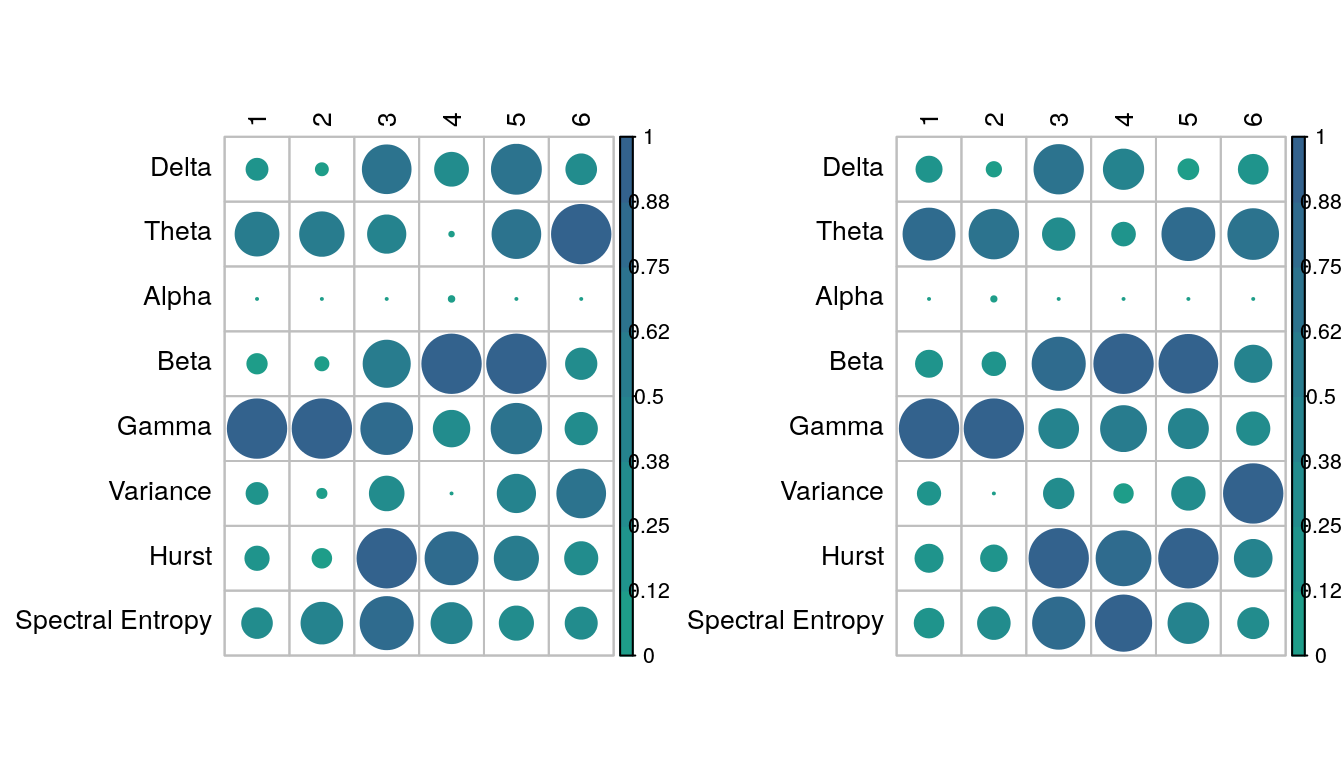
Variable importance (mean-decrease in GINI) for all model and channel combinations. On the left is the model segmented by complexity coefficients A+B. On the right is the model with 8 uniform partitions.
Although the underlying random forest classifier can be highly non-linear the pattern of variable importance is reflected in the differences of distributions of the raw features. The boxplots below show clear differences in the distributions of the relative gamma and theta for channel 1.
knitr::read_chunk("../code/eeg-boxplot-ch1.R") library(dplyr)
library(viridis)
prefix = "eeg"
seed = 2017
chs = 1:6
segch = 4
from_cache = TRUE
window = 240
len = window/2
colnums = c(5:9, 13:15, 21, 19)
feature_df <-readRDS(cache_file("mod_all_features", prefix))
trial_df <- readRDS(cache_file("mod_trial_segments", "eeg"))
df <- do.call(rbind, feature_df)
df <- df %>% cbind(trial_df)
df <- filter(df, window == 240)
palettte <- eegpalette(0.9)[c(1,3)]
# Combine all observation for each channel
# Returns list of 6 data frames, one for each channel
chdf <- apply(df[1:6], 2, function(x) do.call(rbind, x))
colnums <- c(5:9, 13:15)
# names(chdf[[1]])[colnums]
# Add response column
response <- rep(df$response, each = 120)
response_id <- as.factor(c(1,1,1,1,1,2,3,1,
1,1,1,1,1,1,1,1,1,1,1,1,1,
2,3,3,2,3,3,2,3,3))
boxplot_panel(chdf[[1]], response, cex = 0.3)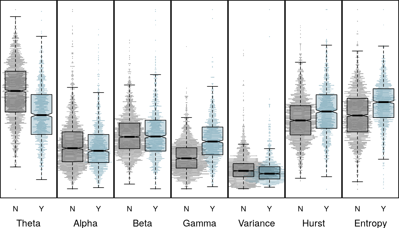
Feature distribution for Channel 1
Channel 1 represents an LFP or local field potential signal, captured from a smaller cluster of neurons in the thalamus. Channel 3 is an iEEG or external EEG sensor placed on the brain surface. For channel 3 the direction of the difference for relative gamma and theta are reversed. Where differences in the beta distribution for seizure an non-seizure trials are not significant for channel 1, for channel three the differences are clear. The difference in distributions is also reflected in the variable importance in the previous plot, as are differences in Hurst and spectral entropy features.
boxplot_panel(chdf[[3]], response, cex = 0.3)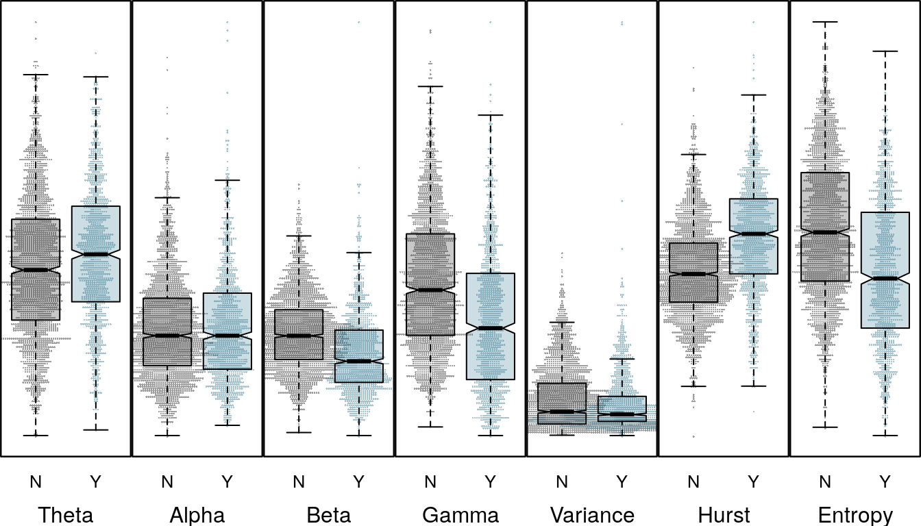
Feature distribution for Channel 3
Session information
sessionInfo()R version 3.4.1 (2017-06-30)
Platform: x86_64-pc-linux-gnu (64-bit)
Running under: Ubuntu 14.04.5 LTS
Matrix products: default
BLAS: /usr/lib/libblas/libblas.so.3.0
LAPACK: /usr/lib/lapack/liblapack.so.3.0
locale:
[1] LC_CTYPE=en_US.UTF-8 LC_NUMERIC=C
[3] LC_TIME=en_US.UTF-8 LC_COLLATE=en_US.UTF-8
[5] LC_MONETARY=en_US.UTF-8 LC_MESSAGES=en_US.UTF-8
[7] LC_PAPER=en_US.UTF-8 LC_NAME=C
[9] LC_ADDRESS=C LC_TELEPHONE=C
[11] LC_MEASUREMENT=en_US.UTF-8 LC_IDENTIFICATION=C
attached base packages:
[1] stats graphics grDevices utils datasets methods base
other attached packages:
[1] corrplot_0.77 caret_6.0-76 lattice_0.20-35
[4] tssegment_0.0.0.9000 randomForest_4.6-12 eegcomplex_0.0.0.1
[7] bindrcpp_0.2 ecomplex_0.0.1 viridis_0.3.4
[10] dplyr_0.7.2 ggplot2_2.2.1
loaded via a namespace (and not attached):
[1] splines_3.4.1 foreach_1.4.3 assertthat_0.2.0
[4] stats4_3.4.1 highr_0.6 yaml_2.1.14
[7] backports_1.0.5 quantreg_5.26 glue_1.1.1
[10] quadprog_1.5-5 pROC_1.9.1 digest_0.6.12
[13] sapa_2.0-2 minqa_1.2.4 colorspace_1.2-6
[16] htmltools_0.3.6 Matrix_1.2-10 plyr_1.8.4
[19] timeDate_3012.100 pkgconfig_2.0.1 devtools_1.13.2
[22] SparseM_1.7 scales_0.4.1 ForeCA_0.2.4
[25] MatrixModels_0.4-1 ifultools_2.0-4 lme4_1.1-13
[28] pracma_2.0.7 git2r_0.19.0 tibble_1.3.3
[31] mgcv_1.8-12 car_2.1-4 withr_1.0.2
[34] nnet_7.3-12 lazyeval_0.2.0 pbkrtest_0.4-6
[37] magrittr_1.5 memoise_1.1.0 evaluate_0.10.1
[40] nlme_3.1-128 MASS_7.3-45 xml2_1.1.1
[43] beeswarm_0.2.3 ggthemes_3.4.0 tools_3.4.1
[46] stringr_1.2.0 munsell_0.4.3 compiler_3.4.1
[49] timeSeries_3022.101.2 fArma_3010.79 rlang_0.1.1
[52] grid_3.4.1 nloptr_1.0.4 iterators_1.0.8
[55] fractaldim_0.8-4 labeling_0.3 rmarkdown_1.6
[58] gtable_0.2.0 ModelMetrics_1.1.0 codetools_0.2-15
[61] fracdiff_1.4-2 gmwm_2.0.0 abind_1.4-3
[64] roxygen2_6.0.1 reshape2_1.4.2 R6_2.2.2
[67] gridExtra_2.2.1 knitr_1.16 bindr_0.1
[70] commonmark_1.2 fBasics_3011.87 rprojroot_1.2
[73] stringi_1.1.5 pdc_1.0.3 parallel_3.4.1
[76] Rcpp_0.12.12 splus2R_1.2-1