Final Topic model
Nathanael Aff
Final model plots
For the final model I used the 40 topic model. The perplexity scores and visualization of the document distribution over topics and color distribution per topic both informed the decision.
- Distribution of themes
- Distribution of themes over time.
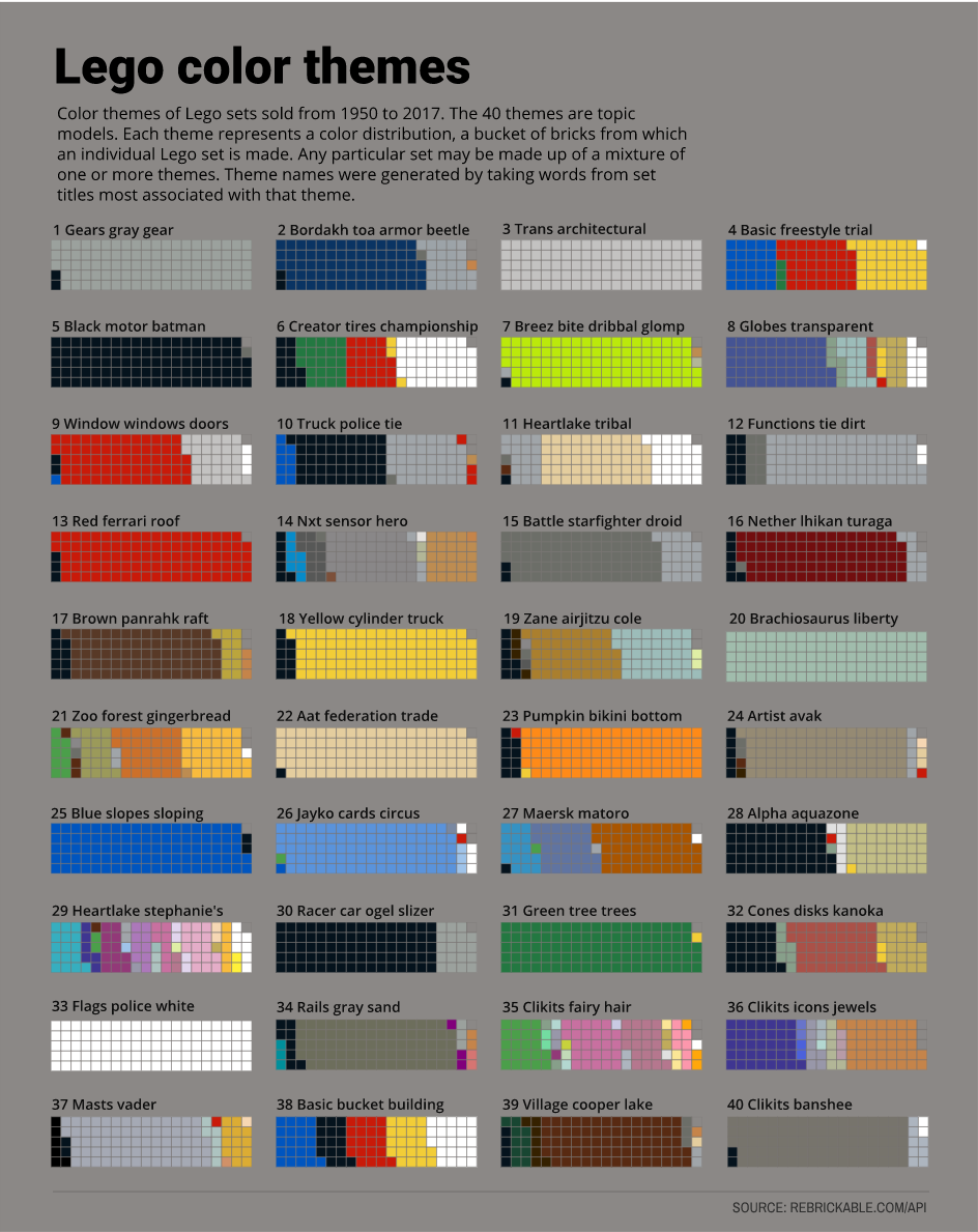
- Color themes
Although themes are a mixture of colors I represented each theme with a single color made of a weighted blend of it’s two colors most associated with that theme.
Theme distribution
devtools::load_all()
knitr::read_chunk(here::here("code", "final-model-plots.R"))
library(dplyr)
library(ggplot2)
# Set model num. Models: 20, 30, 40, 50, 60, 75, 100
create_tables(sample_data = FALSE)Loading table 'set_colors'Loading datasets from CSV files
Assigning themes to theme_df
Assigning full set set inventories to 'set_colors'
Assigning values to total_words
Assigning tidy set and color dataframe to 'set_words'
Creating sparse document term matrix (tm-package) and assigning to 'dtm' lda_models <- get_lda_models()
model_num = 3
topic_num = get_topic_numbers(lda_models)[model_num]
# Label sets by top topic probability
lda_clust <- get_lda_clusters(lda_models)
set_num <- names(lda_clust[model_num, ]$clust[[1]])
set_clust <- tidyr::unnest(lda_clust, clust) %>% mutate(topic_id = clust) %>%
filter(k == 40) %>% mutate(set_num = set_num) %>% left_join(sets_df) %>%
arrange(topic_id) %>% mutate(topic_id = forcats::fct_inorder(factor(topic_id)))
topic_pal <- topic_palette()
# Get count per topic
set_clust <- set_clust %>% count(topic_id) %>% arrange(n)
tpnames <- get_topic_names(lda_models[[model_num]])
tpnames <- tpnames %>% mutate(topic = factor(topic))
# Change palette names to match topic names
names(topic_pal) <- tpnames$topic_name
set_clust <- set_clust %>% left_join(tpnames, by = c(topic_id = "topic"))
# plot
bgcol = "#8B8684"
gg <- set_clust %>% ggplot(aes(x = reorder(topic_name, n), y = n, fill = topic_name,
group = topic_name))
gg <- gg + geom_col(size = 0.8)
gg <- gg + geom_hline(yintercept = c(300, 600, 900), size = 0.5, col = bgcol)
gg <- gg + scale_fill_manual(values = topic_pal)
# gg <- gg + scale_y_continuous(breaks = c(300, 600, 900))
gg <- gg + labs(x = "Theme", y = "Sets in theme", subtitle = "Distribution of themes for all LEGO sets, 1950 to 2017",
title = "LEGO color theme frequency")
gg <- gg + theme_waff()
gg <- gg + coord_flip()
gg <- gg + theme_dark_bar(bgcol = bgcol)
gg <- gg + geom_vline(xintercept = c(300, 600, 900), size = 0.7, col = bgcol)
gg <- gg + theme(legend.position = "none")
gg <- gg + theme(axis.text = element_text(family = "Roboto Condensed", color = "gray5",
face = "plain", size = 7))
gg <- gg + theme(axis.title = element_text(family = "Roboto Condensed", color = "gray1",
face = "bold", size = 9))
gg <- gg + theme(plot.subtitle = element_text(family = "Roboto Condensed", color = "gray10",
face = "plain", size = 9))
gg
LEGO theme timeline
model_num = 3
topic_num = get_topic_numbers(lda_models)[model_num]

# Assumes topic_pal is available
lda_clust <- lda_clust <- get_lda_clusters(lda_models)

# Model with 50 clusters
set_clust <- tidyr::unnest(lda_clust, clust) %>%
              mutate(topic_id = clust) %>%
              filter(k == topic_num) %>%
              mutate(set_num = set_num) %>%
              left_join(sets_df) %>%
              arrange(topic_id) %>%
              mutate(topic_id = forcats::fct_inorder(factor(topic_id)))

topic_pal <- topic_palette()

tpnames <- get_topic_names(lda_models[[model_num]])
tpnames <- tpnames %>% mutate(topic = factor(topic))
# Change palette names to match topic names
names(topic_pal) <- tpnames$topic_name


set_clust <- set_clust %>%
left_join(tpnames, by = c("topic_id" = "topic")) %>%
mutate(topic_name = forcats::fct_inorder(topic_name))

# Get count by year and topic
set_clust %>%
group_by(topic_name, year) %>%
count(topic_id) %>%
ggplot(aes(x = year, y = n,
    group = topic_name,
    color = topic_name)) +
geom_line(aes(color = factor(topic_name)), size = 0.8) +
geom_area(aes(fill = topic_name), alpha = 1) +
scale_color_manual(values = topic_pal) +
scale_fill_manual(values = topic_pal) +
scale_x_continuous(breaks = c(1960, 1980, 2000)) +
labs(x = "",
  y = "Sets in theme",
  subtitle = "Number of sets published per year associated with a color theme",
  title = "LEGO sets per color theme, 1950-2017") +
facet_wrap(~topic_name, nrow = 10) +
theme_scatter(bgcol = bgcol, grid_col = "#c8c6c4") +
theme(
      plot.title = element_text(
        family = "Roboto",
        size = 20,
        face = "bold",
        color = "gray5"
      ),
      plot.subtitle = element_text(
        family = "Roboto Condensed",
        color = "gray15",
        face = "plain",
        size = 11
      ),
      strip.text  = element_text(
        family = "Roboto Condensed",
        face = "plain",
        size = 10,
        color = "gray5"
        ),
      axis.title = element_text(
        family = "Roboto Condensed",
        face = "bold",
        size = 11,
        color = "gray5"
      ),
      axis.text = element_text(
        family = "Roboto Condensed",
        # face = "bold",
        size = 10,
        color = "gray5"
      )) +
theme(legend.position = "none")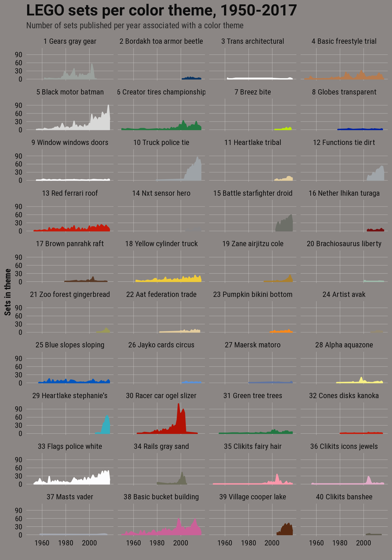
Theme color distributions
knitr::read_chunk(here::here("code", "final-model-grid.R"))library(forcats)
library(purrr)
library(grid)
library(ggplot2)
library(gridExtra)
if(!exists("set_colors")){
cat("Loading data \n")
legolda::load_csv(sample_data = FALSE)
legolda::create_tables()
}
lda_models <- readRDS(here::here("inst", "data", "lda_models_all.RDS"))
model_num = 3
ntopics = lda_models[[model_num]]@k
# Get top 2 colors for each topic
lda_models <- lda_models %>%
purrr::map(function(x) {
class(x) <- "LDA"
x
})
# Total frequency used in relevance score
word_freq <- set_colors %>%
count(rgba) %>%
mutate(percent = n / nrow(set_colors))
lambda = 0.5
nterms = 50
top_colors <- top_terms(lda_models[[model_num]], lambda, nterms, word_freq) %>%
mutate(topic_name = forcats::fct_inorder(factor(topic_name))) %>%
mutate(rep = round(beta*100)) %>%
select(topic, term, rep)
# Expand by the beta weight of the color
top_colors <- top_colors[rep(seq(nrow(top_colors)), top_colors$rep), 1:3]
# Get counts for waffle plot. Wrapper needs name in name column
tp <- top_colors %>% count(topic, term) %>%
rename(count = n)
tpnames <- get_topic_names(lda_models[[model_num]])
tp <- tp %>% left_join(tpnames) %>%
rename(name = topic_name)
waff_topic <- function(data, ntopic, col) {
p <- data %>% filter(topic == ntopic)
wp <- waffle2(
p$count,
title = p$name,
colors = p$term,
rows = 5, size = 0.3,
grout_color = col)
# wp <- wp + theme_waff(col)
wp <- wp + theme(legend.position = "none")
wp <- wp + theme(
# panel.spacing = unit(1.2, "lines"),
plot.title = element_text(
size = 16,
# family = "Roboto Condensed",
face = "plain",
color = "gray5"
),
plot.subtitle = element_text(
color = "gray10",
face = "plain",
size = 11
),
axis.title = element_text(
size = 11 ,
color = "gray15"
),
axis.text = element_blank(),
plot.caption = element_text(
face = "italic",
size = 9,
color = "gray25"
)
)
# wp <- wp + theme_waff(bgcol = col, modify_text = FALSE)
# wp <- wp + theme(plot.title = element_text(size = 10, face = "bold"))
wp
}
bgcol <- "#787472"
pp <- map(1:ntopics, ~waff_topic(data = tp, ntopic = .x, col = bgcol))
pdf(here::here("docs", "figure", "final-grid-plot.pdf"), width = 13, height = 15)
grid.draw(
grobTree(
rectGrob(gp=gpar(fill= bgcol, lwd=0)),
do.call(arrangeGrob, c(pp, ncol = 4)
)))
dev.off()