Cross validation on perplexity

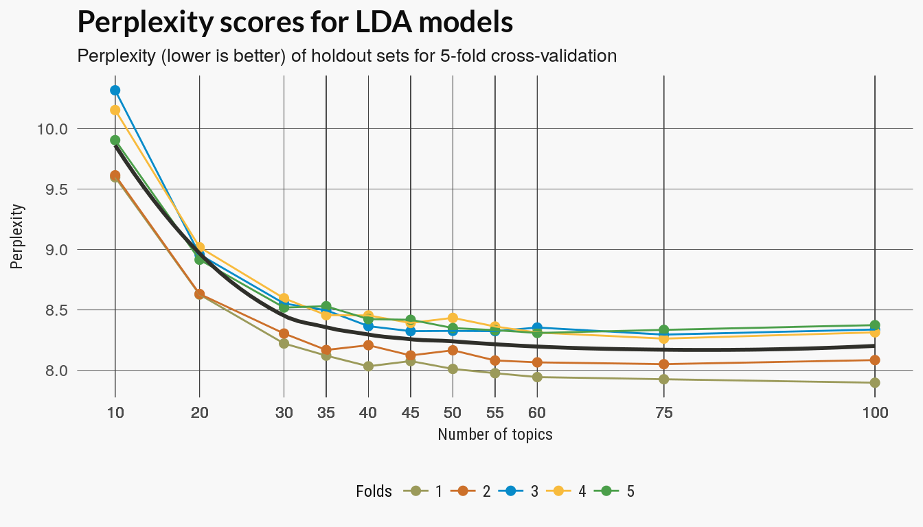
The LDA model learns to posterior distributions which are the optimization routine’s best guess at the distributions that generated the data. One method to test how good those distributions fit our data is to compare the learned distribution on a training set to the distribution of a holdout set. Perplexity is one measure of the difference between estimated topic distributions on documents.

We cast the set_word table to a document term matrix using the tidytext function. This returns adocumentTermMatrix object from the tm package. The LDA function we use is from the topicmodels package. It has a variational expectation maximation method and a Gibbs sampling method and I used the former.

Loading datasets from CSV files 
Assigning themes to theme_df 
Assigning full set set inventories to 'set_colors' 
Assigning values to total_words
Assigning tidy set and color dataframe to 'set_words' 
Creating sparse document term matrix (tm-package) and assigning to 'dtm' 

perplexities <- readRDS(here::here("inst", "data", "perplexity_all.RDS"))

perplexities %>% ggplot(aes(n_topic, perplexity)) + geom_point(aes(colour = fold), 
    size = 2) + geom_line(aes(n_topic, perplexity, group = fold, colour = fold)) + 
    scale_color_manual(values = pal21(), guide = guide_legend(title = "Folds")) + 
    geom_smooth(se = FALSE, colour = "#2f2f2a") + scale_x_continuous(breaks = perplexities$n_topic) + 
    labs(x = "Number of topics", y = "Perplexity", title = "Perplexity scores for LDA models", 
        subtitle = "Perplexity (lower is better) of holdout sets for 5-fold cross-validation") + 
    legolda::theme_scatter(bgcol = "#f8f8f8")

ntopics <- c(20, 30, 35, 40, 50, 75, 100)
# Train LDA models on full data set
if (!from_cache) {
    lda_models <- c(20, 30, 35, 40, 50, 75, 100) %>% purrr::map(LDA, x = dtm, 
        control = list(seed = 1))
}

ldatuning topic scores

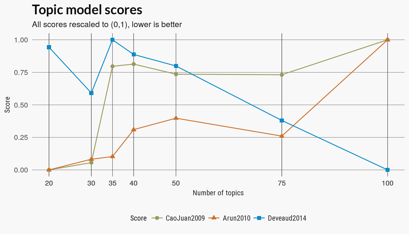
The ldatuning package has several other metrics of the quality of the topic models. I have modified the main function from the package to only return the scores. (The original package computes the models first and then the scores).

knitr::read_chunk(here::here("code", "ldatuning-scores.R"))

lda_models <- readRDS(here::here("inst", "data", "lda_models_all.RDS"))
lda_metrics <- legolda::score_models(lda_models, dtm, topics = ntopics)

plot_lda_scores(lda_metrics, title)

Topic coherence

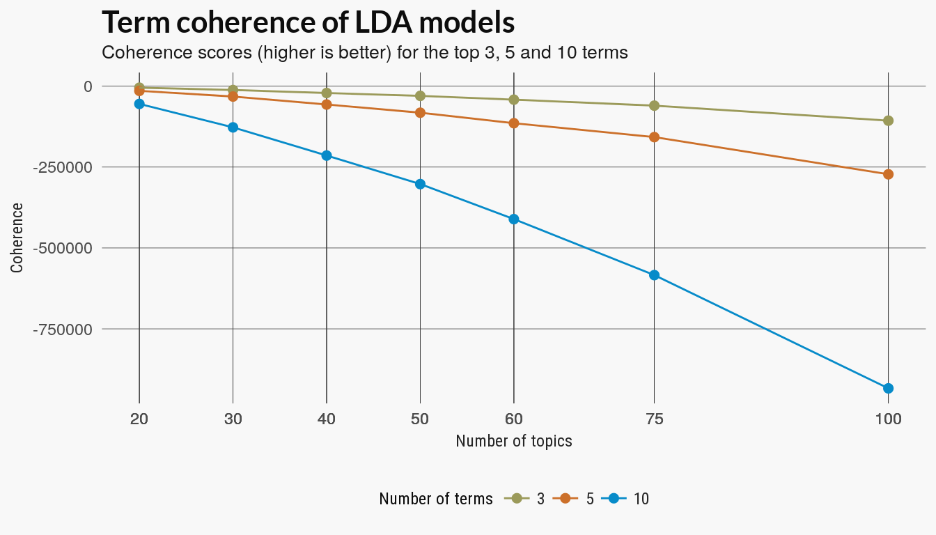
There are several version of topic coherence which measure the pairwise strength of the relationship of the top terms in a topic model. Given some score where a larger value indicates a stronger relation ship between two words \(w_i, w_j\), a generic coherence score is the sum over the top terms in a topic model:
\[ \sum_{w_i, w_j \in W_t} \text{Score}(w_i, w_j), \] with top terms \(W_t\) for each topic \(t\).

The coherence score used in the SpeedReader coherence function just uses the internal coherence of the top terms. I compared the scores for the top 3, 5 and 10 terms.

coh_tbl <- readRDS(here::here("inst", "data", "coherence.RDS"))
coh_tbl <- coh_tbl %>% mutate(nterms = forcats::fct_inorder(nterms))

# TODO: sort number of terms in order

coh_tbl %>% ggplot(aes(x = ntopics, y = coherence, group = nterms)) + geom_point(aes(colour = nterms, 
    group = nterms), size = 2) + geom_line(aes(color = nterms)) + scale_color_manual(values = pal21(), 
    guide = guide_legend(title = "Number of terms")) + scale_x_continuous(breaks = coh_tbl$ntopics) + 
    labs(x = "Number of topics", y = "Coherence", title = "Term coherence of LDA models", 
        subtitle = "Coherence scores (higher is better) for the top 3, 5 and 10 terms") + 
    theme_scatter(bgcol = "#f8f8f8")

Cluster scoring

We can also treat the LDA models as clustering the LEGO sets. We can assign the LEGO set to the color topic which has the highest value for that document; This is the topic that is most responsible for generating the document.

The previous plot should indicate whether documents are getting strongly associated with a topic or if topics are to evenly distributed over all documents.

Topic Distribution

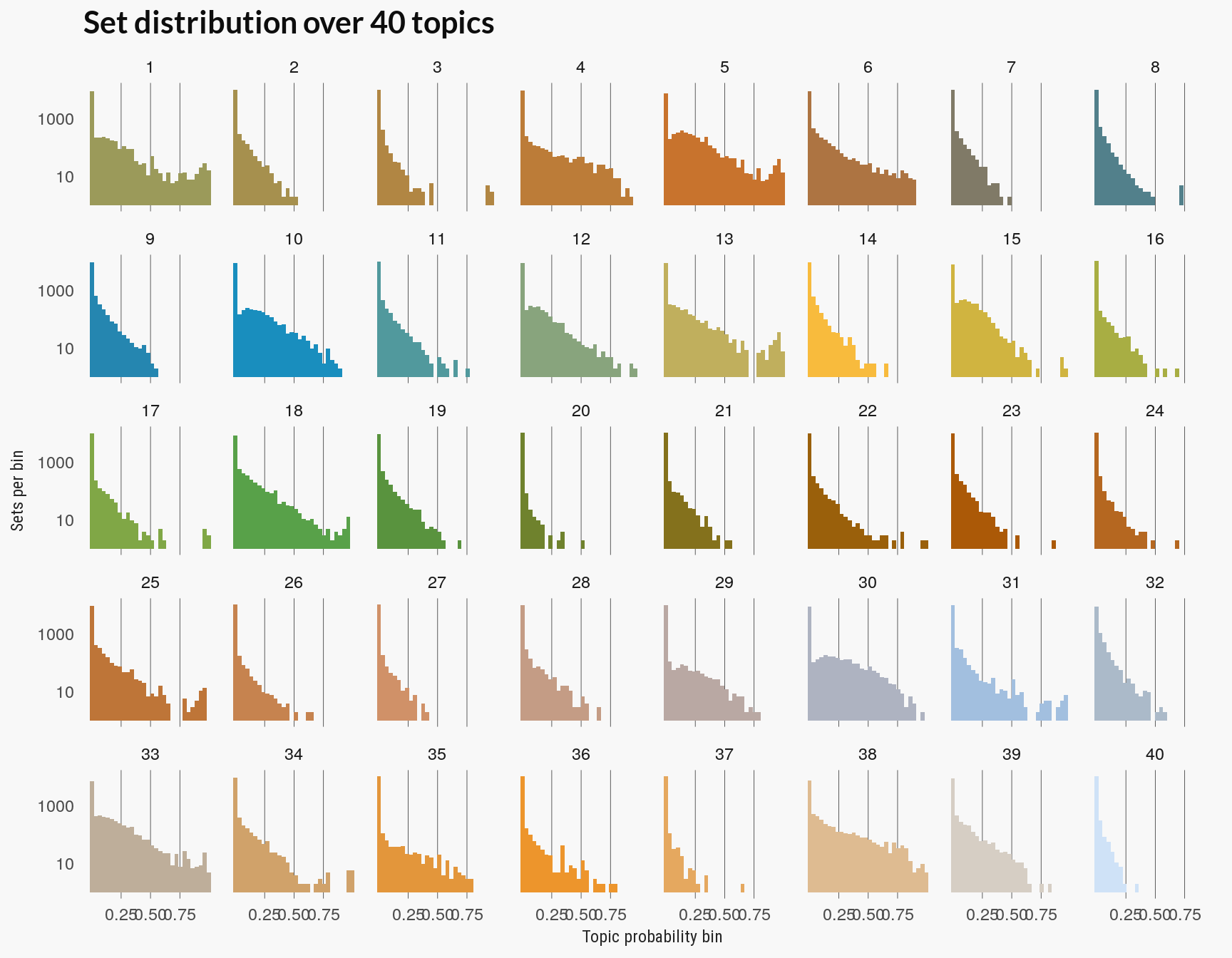
Another way to evaluate the quality of the topic models is to see how well documents are sorted into topics. This example follows a this section from the tidy text mining book.

The topic model’s gamma matrix has the distribution of topics over models: \[ \text{gamma} = p(t|d) \] for topic \(t\) and document \(d\).

The plot below visualizes this as how the topics are distributed over the probability bins for each topic. If too many topics have sets or documents in the low probability bins then you may have too high a number of topics since few documents are being strongly associated with any topic.

Following the tidytext book, look at the distribution over topics.